Exponential smoothing
Exponential smoothing assigns exponentially decreasing weights to past observations: recent values matter more than distant ones. It is one of the most widely used forecasting methods in practice due to its simplicity, adaptability, and strong empirical performance, particularly for short-term horizons.
Simple exponential smoothing (SES)
Used for series with no trend and no seasonality. The smoothed value \(\hat{y}_{t+1}\) is a weighted average of the current observation and the previous forecast:
\[\hat{y}_{t+1} = \alpha y_t + (1-\alpha)\hat{y}_t, \qquad 0 < \alpha \leq 1\]
Expanding recursively:
\[\hat{y}_{t+1} = \alpha y_t + \alpha(1-\alpha)y_{t-1} + \alpha(1-\alpha)^2 y_{t-2} + \cdots\]
Each past observation receives weight \(\alpha(1-\alpha)^j\) at lag \(j\). Weights decrease geometrically: observation from 5 periods ago receives weight \(\alpha(1-\alpha)^5\).
The smoothing parameter \(\alpha\):
- \(\alpha\) close to 1: high weight on the most recent observation, little memory. Reacts quickly but is noisy.
- \(\alpha\) close to 0: slow adaptation, heavy smoothing. Reacts slowly to changes.
- Optimal \(\alpha\) is estimated by minimizing the sum of squared one-step forecast errors.
SES forecasts are flat: \(\hat{y}_{T+h} = \hat{y}_{T+1}\) for all \(h > 1\). It cannot extrapolate a trend.
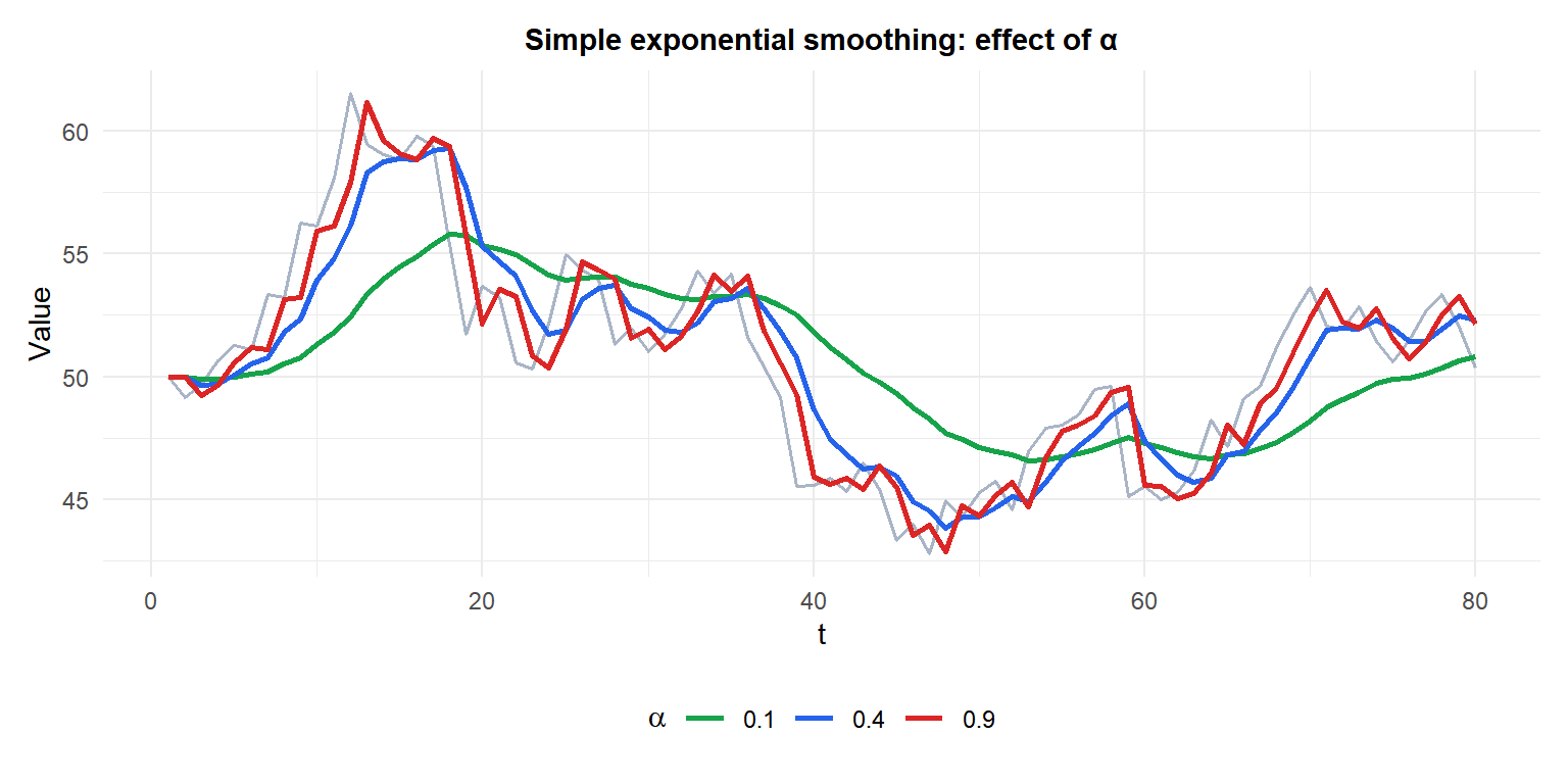
High \(\alpha\) (red) tracks the data closely but is noisy. Low \(\alpha\) (green) is smoother but slower to adapt to real changes.
Double exponential smoothing (Holt’s method)
Extends SES to series with a trend but no seasonality. Two smoothing equations: one for the level \(\ell_t\) and one for the trend \(b_t\):
\[\ell_t = \alpha y_t + (1-\alpha)(\ell_{t-1} + b_{t-1})\]
\[b_t = \beta(\ell_t - \ell_{t-1}) + (1-\beta)b_{t-1}\]
\[\hat{y}_{t+h} = \ell_t + h \cdot b_t\]
\(\alpha \in (0,1)\) smooths the level; \(\beta \in (0,1)\) smooths the trend. The \(h\)-step forecast extrapolates the estimated trend linearly from the last smoothed level.
Holt’s method assumes a constant additive trend: long-horizon forecasts diverge linearly. For damped trends (which often forecast better), a damping parameter \(\phi \in (0,1)\) is added: \(\hat{y}_{t+h} = \ell_t + (\phi + \phi^2 + \cdots + \phi^h)b_t\).
Triple exponential smoothing (Holt-Winters)
Adds a seasonal component to Holt’s method. Two variants:
Additive (constant seasonal amplitude):
\[\ell_t = \alpha(y_t - s_{t-m}) + (1-\alpha)(\ell_{t-1} + b_{t-1})\]
\[b_t = \beta(\ell_t - \ell_{t-1}) + (1-\beta)b_{t-1}\]
\[s_t = \gamma(y_t - \ell_{t-1} - b_{t-1}) + (1-\gamma)s_{t-m}\]
\[\hat{y}_{t+h} = \ell_t + h \cdot b_t + s_{t+h-m}\]
Multiplicative (seasonal amplitude proportional to level): replace additive operations with multiplicative ones. Use when seasonal swings grow with the level.
\(m\) is the season length (12 for monthly, 4 for quarterly). The covered in detail in the Holt-Winters post.
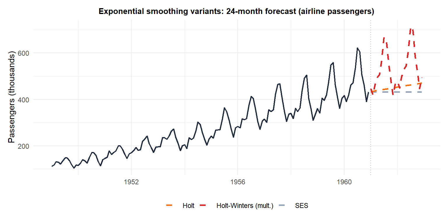
SES (grey) produces a flat forecast. Holt (orange) captures the trend but not seasonality. Holt-Winters multiplicative (red) captures both trend and growing seasonal amplitude: the most accurate for this series.
The ETS framework
All exponential smoothing methods are special cases of the ETS (Error, Trend, Seasonality) framework, which provides a unified state space representation:
- Error: additive (A) or multiplicative (M).
- Trend: none (N), additive (A), additive damped (Ad).
- Seasonality: none (N), additive (A), multiplicative (M).
Examples: ETS(A,N,N) = SES; ETS(A,A,N) = Holt’s method; ETS(M,A,M) = multiplicative Holt-Winters.
The ETS framework allows model selection by AIC and provides proper prediction intervals via the state space representation. It is implemented in R’s ets() function which selects the best model automatically.
⚠️ Exponential smoothing is not suitable for all series
Exponential smoothing works best for series with a stable structure (level, trend, seasonality) that changes slowly. It can underperform for:
- Series with structural breaks or sudden changes in trend.
- Series where the future is driven by external variables (use ARIMAX or regression instead).
- Series with complex autocorrelation patterns that need explicit AR/MA modelling.
For series with clear external drivers (e.g., sales driven by promotions, demand driven by temperature), regression-based or ARIMAX models are more appropriate.
💡 Exponential smoothing in R
library(forecast)

# Simple exponential smoothing
ses(y, h = 12)

# Holt's method (trend, no seasonality)
holt(y, h = 12, damped = TRUE)  # damped trend often forecasts better

# Holt-Winters
hw(y, h = 12, seasonal = "multiplicative")  # or "additive"

# Automatic ETS model selection
fit <- ets(y)
summary(fit)
forecast(fit, h = 12)
The ets() function selects the best ETS model by AIC, choosing among all combinations of error, trend and seasonal components.

