EGARCH model
EGARCH (Exponential GARCH), introduced by Nelson (1991), extends GARCH to capture the leverage effect: negative return shocks increase future volatility more than positive shocks of the same magnitude. This asymmetry is one of the most robust empirical regularities in equity markets and cannot be captured by standard GARCH.
The leverage effect
In equity markets, a negative return (stock price falls) increases the firm’s financial leverage (debt-to-equity ratio rises), making future cash flows riskier. This mechanically increases volatility. Empirically, the effect is stronger and more persistent than the symmetric response predicted by GARCH:
- A 2% daily loss increases next-day volatility more than a 2% daily gain.
- The asymmetry is well-documented for individual stocks, equity indices, and many commodity markets.
- It is absent or reversed in some asset classes (e.g., volatility itself tends to be positively skewed).
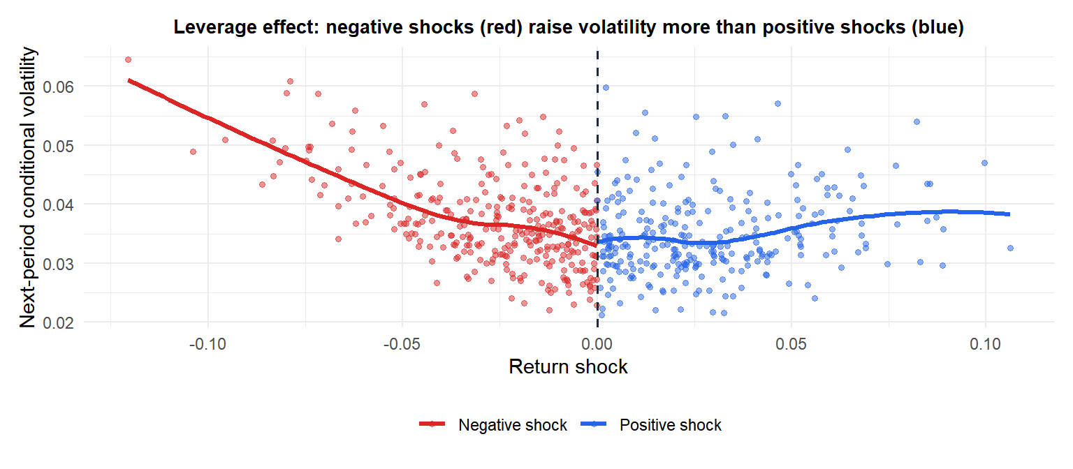
For negative shocks (red), next-period volatility rises steeply. For positive shocks of the same size (blue), volatility rises less. GARCH would produce a symmetric U-shaped curve; EGARCH produces an asymmetric one.
The EGARCH model
Nelson (1991) modeled the log of conditional variance to avoid positivity constraints:
\[\log\sigma_t^2 = \omega + \sum_{j=1}^p \beta_j \log\sigma_{t-j}^2 + \sum_{i=1}^q \left[\alpha_i z_{t-i} + \gamma_i\left(|z_{t-i}| - E[|z_{t-i}|]\right)\right]\]
\[z_t = \frac{\varepsilon_t}{\sigma_t} \sim \text{i.i.d.}(0,1)\]
For the standard EGARCH(1,1):
\[\log\sigma_t^2 = \omega + \beta_1 \log\sigma_{t-1}^2 + \alpha_1 z_{t-1} + \gamma_1\left(|z_{t-1}| - \sqrt{2/\pi}\right)\]
The three key terms after \(\omega\):
- \(\beta_1 \log\sigma_{t-1}^2\): persistence. Same role as \(\beta\) in GARCH.
- \(\gamma_1(|z_{t-1}| - E[|z_{t-1}|])\): size effect. Large shocks (positive or negative) increase log-variance.
- \(\alpha_1 z_{t-1}\): sign effect. Negative \(z_{t-1}\) (bad news) increases log-variance by \(|\alpha_1|\); positive \(z_{t-1}\) decreases it. The leverage effect corresponds to \(\alpha_1 < 0\).
The total effect of a shock \(z_{t-1}\) on \(\log\sigma_t^2\):
\[g(z_{t-1}) = \begin{cases} (\alpha_1 + \gamma_1)z_{t-1} - \gamma_1 E[|z|] & z_{t-1} > 0 \\ (\alpha_1 - \gamma_1)z_{t-1} - \gamma_1 E[|z|] & z_{t-1} < 0 \end{cases}\]
For \(\alpha_1 < 0\): negative shocks have slope \(|\alpha_1| + \gamma_1\) (steeper) and positive shocks have slope \(\gamma_1 - |\alpha_1|\) (flatter).
GARCH vs EGARCH: the news impact curve
The news impact curve (NIC) plots \(\sigma_t\) as a function of \(\varepsilon_{t-1}\), holding \(\sigma_{t-1}^2\) constant at its long-run value. It shows the asymmetry explicitly.
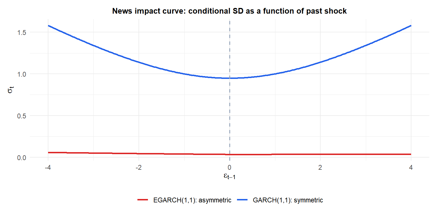
GARCH (blue) is symmetric: shocks of \(-2\) and \(+2\) produce the same \(\sigma_t\). EGARCH (red) is asymmetric: negative shocks produce higher volatility than positive shocks of the same magnitude.
Advantages over GARCH
EGARCH has two important technical advantages over standard GARCH:
No positivity constraints. Since EGARCH models \(\log\sigma_t^2\), no restrictions on the parameters are needed to ensure \(\sigma_t^2 > 0\). Standard GARCH requires \(\omega > 0\), \(\alpha_i \geq 0\), \(\beta_j \geq 0\), which can be binding near the boundary.
Captures asymmetry. The \(\alpha_1\) parameter directly measures the leverage effect. A significantly negative \(\hat{\alpha}_1\) confirms that bad news has a larger impact on volatility than good news.
Fitting EGARCH(1,1)
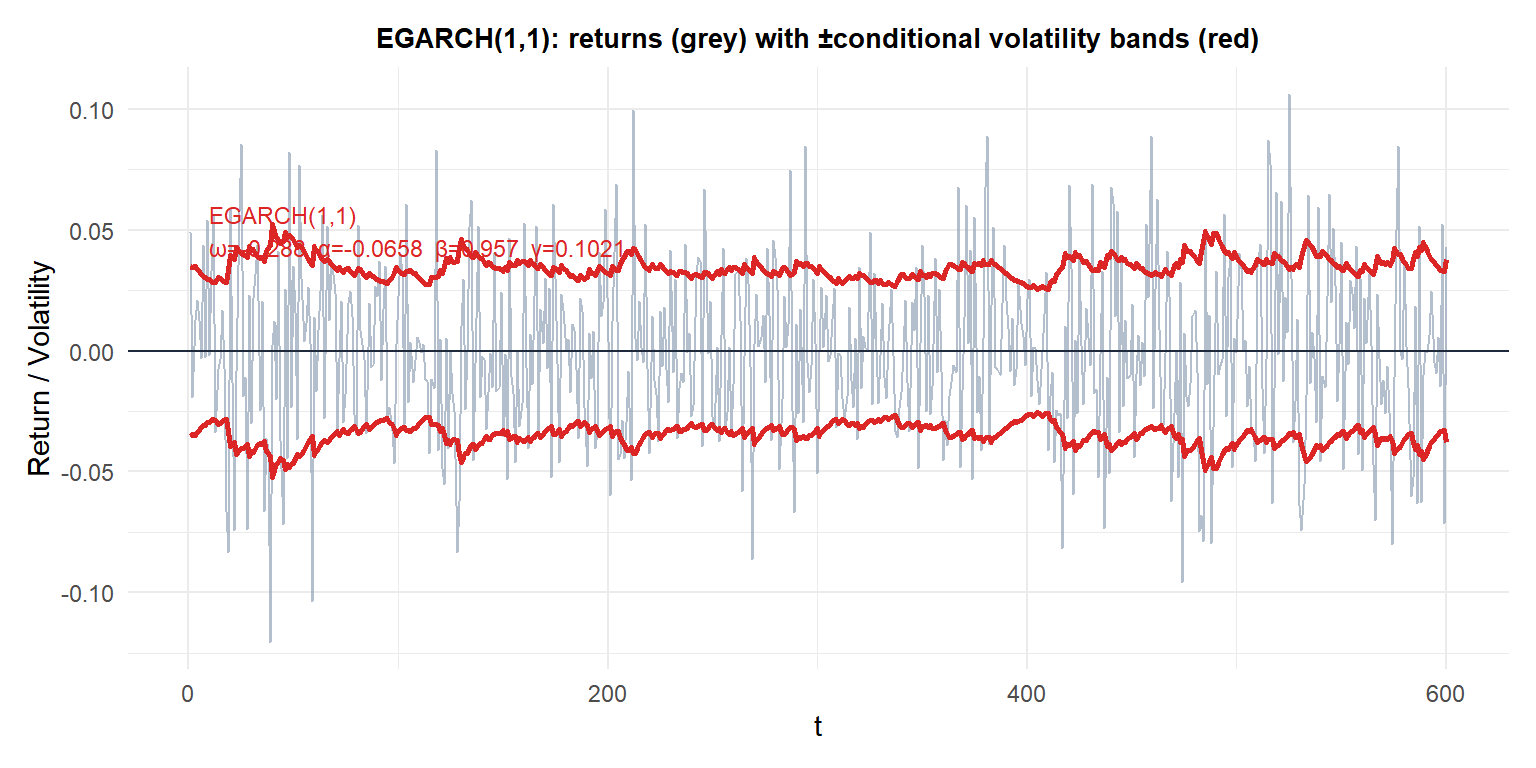
The negative \(\alpha\) coefficient confirms the leverage effect: following negative return shocks, the volatility bands widen more than after equivalent positive shocks.
⚠️ Interpreting EGARCH coefficients requires care
The sign conventions for \(\alpha\) and \(\gamma\) vary across software packages:
- In
rugarch: \(\alpha_1\) is the sign effect and \(\gamma_1\) is the size effect. The leverage effect corresponds to \(\alpha_1 < 0\). - In some textbooks: the parameterization uses \(\theta\) and \(\kappa\) instead, with different sign conventions.
Always check the documentation of the package you use and verify that \(\hat{\sigma}_t\) rises more after negative shocks by plotting the news impact curve or examining conditional volatility around known market stress events.
When to use EGARCH vs GARCH
| Situation | Recommended |
|---|---|
| Equity returns (stocks, indices) | EGARCH (leverage effect expected) |
| Symmetric assets (FX, commodities) | GARCH or GJR-GARCH |
| Positive-only series (interest rates) | Log-GARCH or EGARCH |
| Quick benchmark | GARCH(1,1) first, then test for asymmetry |
Test whether asymmetry is significant: fit both GARCH and EGARCH and compare AIC, or test \(H_0: \alpha_1 = 0\) in the EGARCH fit.
💡 EGARCH in R
library(rugarch)

spec_eg <- ugarchspec(
  variance.model     = list(model = "eGARCH", garchOrder = c(1,1)),
  mean.model         = list(armaOrder = c(0,0), include.mean = TRUE),
  distribution.model = "std"
)

fit_eg <- ugarchfit(spec_eg, data = returns)
coef(fit_eg)        # omega, alpha1 (sign), beta1, gamma1 (size), shape
sigma(fit_eg)       # conditional volatility
newsimpact(fit_eg)  # news impact curve data

# Compare GARCH vs EGARCH by AIC
infocriteria(fit_garch)[1]
infocriteria(fit_eg)[1]
