Correspondence analysis
Correspondence Analysis (CA) is the PCA equivalent for contingency tables. It finds a low-dimensional representation of the rows and columns of a two-way frequency table that preserves the chi-square distances between profiles. The result is a biplot where rows and columns close to each other are associated, and rows or columns near the origin have unremarkable profiles.
The contingency table and profiles
CA starts with a contingency table \(\mathbf{N}\) of size \(I \times J\), where \(n_{ij}\) is the frequency of row category \(i\) and column category \(j\). Define:
- \(n = \sum_{i,j} n_{ij}\): grand total.
- \(\mathbf{P} = \mathbf{N}/n\): correspondence matrix (relative frequencies).
- \(r_i = \sum_j p_{ij}\): row marginals.
- \(c_j = \sum_i p_{ij}\): column marginals.
The row profile of row \(i\) is \(\mathbf{f}_i = (p_{i1}/r_i, \ldots, p_{iJ}/r_i)\): the conditional distribution of columns given row \(i\). The column profile of column \(j\) is \(\mathbf{g}_j = (p_{1j}/c_j, \ldots, p_{Ij}/c_j)\).
CA finds coordinates for rows and columns such that:
- Rows (columns) with similar profiles are close together.
- The distance used is the chi-square distance, which weights each column (row) by the inverse of its marginal frequency, giving more weight to rare categories.
The chi-square distance between rows \(i\) and \(i'\):
\[d^2_\chi(i,i') = \sum_j \frac{1}{c_j}\left(\frac{p_{ij}}{r_i} - \frac{p_{i'j}}{r_{i'}}\right)^2\]
SVD decomposition
CA applies SVD to the matrix of standardized residuals:
\[s_{ij} = \frac{p_{ij} - r_i c_j}{\sqrt{r_i c_j}}\]
The numerator \(p_{ij} - r_i c_j\) is the deviation from independence: if rows and columns were independent, the expected proportion would be \(r_i c_j\). The denominator standardizes by the expected count.
\[\mathbf{S} = \mathbf{U}\boldsymbol{\Sigma}\mathbf{V}^T\]
The row coordinates (scores) are \(\mathbf{F} = \mathbf{D}_r^{-1/2}\mathbf{U}\boldsymbol{\Sigma}\) and the column coordinates are \(\mathbf{G} = \mathbf{D}_c^{-1/2}\mathbf{V}\boldsymbol{\Sigma}\), where \(\mathbf{D}_r\) and \(\mathbf{D}_c\) are diagonal matrices of row and column marginals.
The squared singular values \(\sigma_k^2\) are the principal inertias: they measure how much of the total chi-square statistic is captured by each dimension. The total inertia equals \(\chi^2/n\), where \(\chi^2\) is the chi-square statistic for the contingency table.
Example: smoking habits by job
A survey records smoking habits (None, Light, Medium, Heavy) by job category (Senior Manager, Junior Manager, Senior Employee, Junior Employee, Secretary).
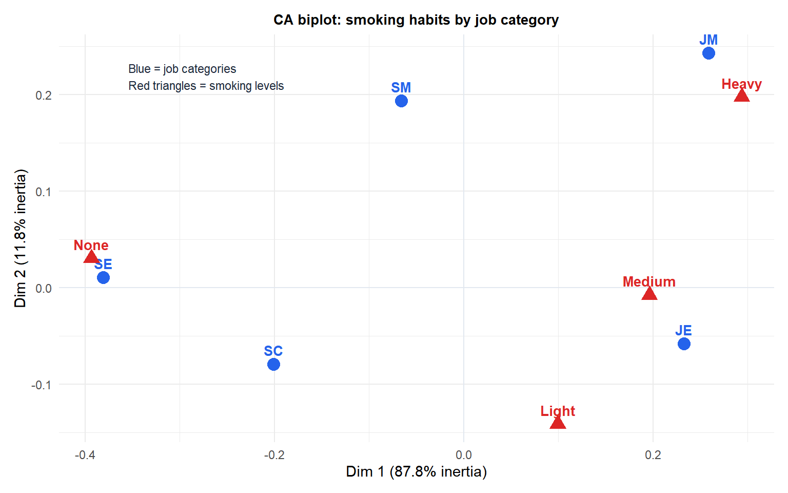
SM = Senior Manager, JM = Junior Manager, SE = Senior Employee, JE = Junior Employee, SC = Secretary. Junior Employees appear close to Heavy smoking; Senior Managers are closer to None. The first dimension separates light from heavy smokers; the second separates managerial from non-managerial roles.
Inertia and how many dimensions
Total inertia = \(\chi^2/n\): measures the total association between rows and columns. Zero inertia means rows and columns are independent. High inertia means strong association.
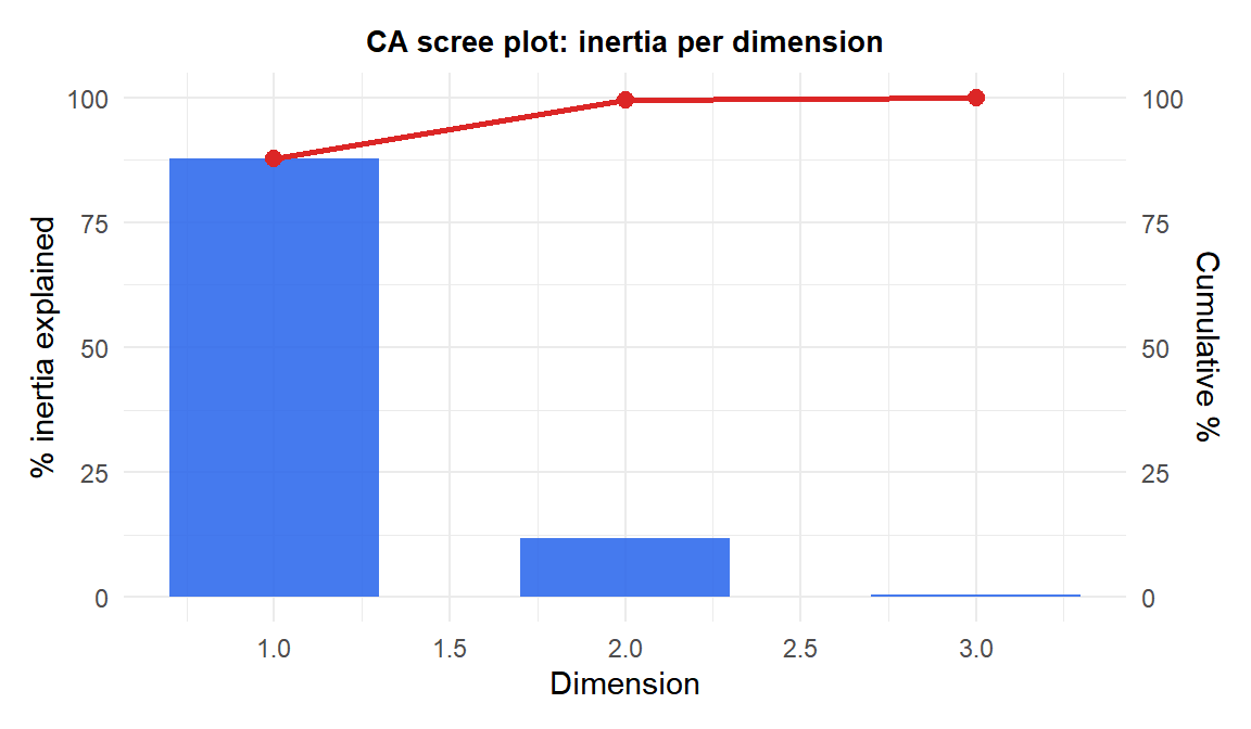
Each dimension captures a fraction of the total inertia (analogous to explained variance in PCA). A scree plot of the principal inertias helps decide how many dimensions to retain.
Reading the biplot
Three rules for interpreting a CA biplot:
Rule 1: rows close together have similar column profiles. Two job categories close together have similar smoking distributions.
Rule 2: columns close together appear in similar row profiles. Two smoking levels close together tend to characterize the same job categories.
Rule 3: a row point near a column point indicates association. A job category near “Heavy” means that category over-represents heavy smokers relative to the average.
Rule 4: distance from the origin. Points near the origin have profiles close to the average (uninteresting); points far from the origin have unusual profiles and drive the dimensions.
⚠️ Row-column proximity requires caution
In a standard CA biplot (symmetric map), the exact distance between a row point and a column point is not directly interpretable as a chi-square distance. The biplot projects both rows and columns in the same space for visual convenience, but the formal chi-square distances are defined separately for rows and for columns.
For a fully interpretable distance between rows and columns use an asymmetric biplot: plot one set of profiles as points and the other as coordinates in that profile space. The FactoMineR function fviz_ca_biplot(asymmetric=TRUE) does this.
Multiple Correspondence Analysis (MCA)
CA handles two categorical variables. Multiple Correspondence Analysis (MCA) extends this to three or more variables. Each individual is described by several categorical variables; MCA finds a low-dimensional space where:
- Individuals who gave similar answers are close together.
- Categories that were often chosen together are close together.
- Categories close to an individual means that individual tends to choose that category.
MCA is equivalent to CA applied to the indicator matrix (a binary matrix with one column per category and one row per individual). It is widely used in survey analysis and market research.
💡 Correspondence analysis in R
library(FactoMineR)
library(factoextra)

# CA on a contingency table
ca_res <- CA(contingency_table, ncp=5, graph=FALSE)
summary(ca_res)          # inertia per dimension
ca_res$eig               # eigenvalues and % inertia
ca_res$row$coord         # row coordinates
ca_res$col$coord         # column coordinates

# Biplot
fviz_ca_biplot(ca_res, repel=TRUE)

# Scree plot
fviz_screeplot(ca_res)

# Contribution of rows/columns to each dimension
fviz_contrib(ca_res, choice="row", axes=1)
fviz_contrib(ca_res, choice="col", axes=1)

# MCA for multiple categorical variables
mca_res <- MCA(df_survey, graph=FALSE)
fviz_mca_biplot(mca_res, repel=TRUE)
