Estimation of a population variance
The sample variance \(S^2\) is the standard point estimator for the population variance \(\sigma^2\). Its key feature is the division by \(n-1\) instead of \(n\), which corrects a systematic bias that arises from estimating the mean from the same data.
The estimator: sample variance
Given a sample \(x_1, x_2, \ldots, x_n\) with sample mean \(\bar{x}\), the sample variance is:
\[S^2 = \frac{1}{n-1} \sum_{i=1}^{n} (x_i - \bar{x})^2\]
This is an unbiased estimator of \(\sigma^2\): \(E[S^2] = \sigma^2\).
The alternative estimator, obtained by dividing by \(n\), is the maximum likelihood estimator (MLE):
\[\hat{\sigma}^2_{\text{MLE}} = \frac{1}{n} \sum_{i=1}^{n} (x_i - \bar{x})^2\]
The MLE is biased: \(E[\hat{\sigma}^2_{\text{MLE}}] = \frac{n-1}{n}\sigma^2 < \sigma^2\).
Why divide by \(n-1\)?
The intuition: when we compute deviations \((x_i - \bar{x})\), we use \(\bar{x}\) instead of the unknown \(\mu\). The sample mean \(\bar{x}\) is always at the center of the data, so the deviations from \(\bar{x}\) tend to be slightly smaller than the deviations from \(\mu\). This causes \(\frac{1}{n}\sum(x_i-\bar{x})^2\) to systematically underestimate \(\sigma^2\).
More formally: the \(n\) deviations \((x_i - \bar{x})\) must sum to zero (because \(\sum(x_i - \bar{x}) = 0\)), so only \(n-1\) of them are free to vary. The divisor \(n-1\) reflects this loss of one degree of freedom.
Suppose the true population has \(\sigma^2 = 10\). We repeatedly take samples of size \(n = 5\) and compute both estimators.
In the long run (across many samples):
\[E\!\left[\frac{1}{5}\sum(x_i-\bar{x})^2\right] = \frac{4}{5} \times 10 = 8 \quad \text{(underestimates by 20\%)}\]
\[E\!\left[\frac{1}{4}\sum(x_i-\bar{x})^2\right] = 10 \quad \text{(correct on average)}\]
For small samples (\(n = 5\)), the bias of the MLE is 20%. For \(n = 100\) it is only 1%, which is why the distinction matters more in small samples.
Sampling distribution of \(S^2\)
The key result connecting \(S^2\) to the chi-squared distribution: if the population is normal, then:
\[\frac{(n-1)S^2}{\sigma^2} \sim \chi^2(n-1)\]
This result has two uses: it confirms that \(S^2\) is unbiased (since \(E[\chi^2(n-1)] = n-1\), giving \(E[S^2] = \sigma^2\)), and it is the foundation for confidence intervals and hypothesis tests about \(\sigma^2\).
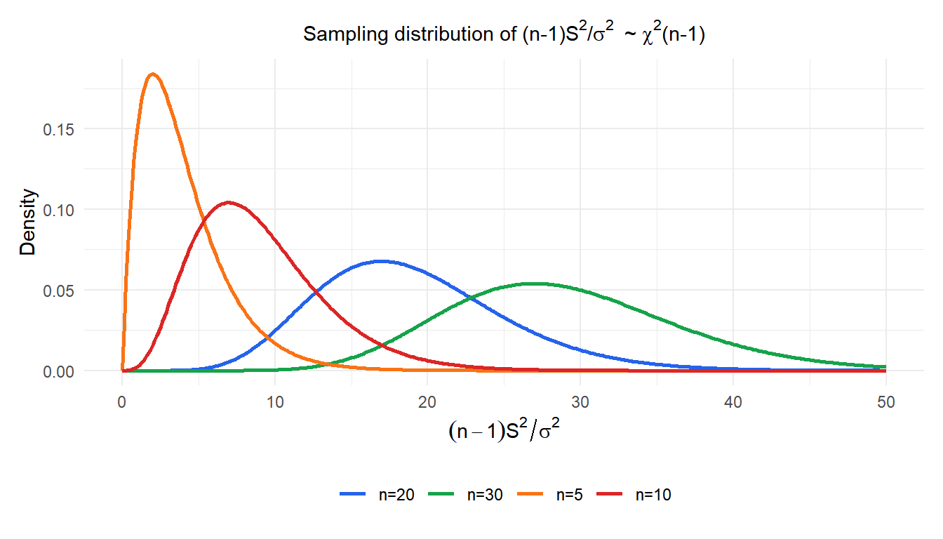
⚠️ The chi-squared distribution is not symmetric
Unlike the sampling distribution of \(\bar{X}\), the distribution of \(S^2\) is always right-skewed. This has two practical consequences:
- Confidence intervals for \(\sigma^2\) are not symmetric around \(S^2\): the upper bound is further from \(S^2\) than the lower bound.
- The skewness is more pronounced for small \(n\) and disappears slowly as \(n\) grows. For small samples, the assumption of normality in the population is important: the chi-squared result only holds exactly when the population is normal.
Comparing the two estimators
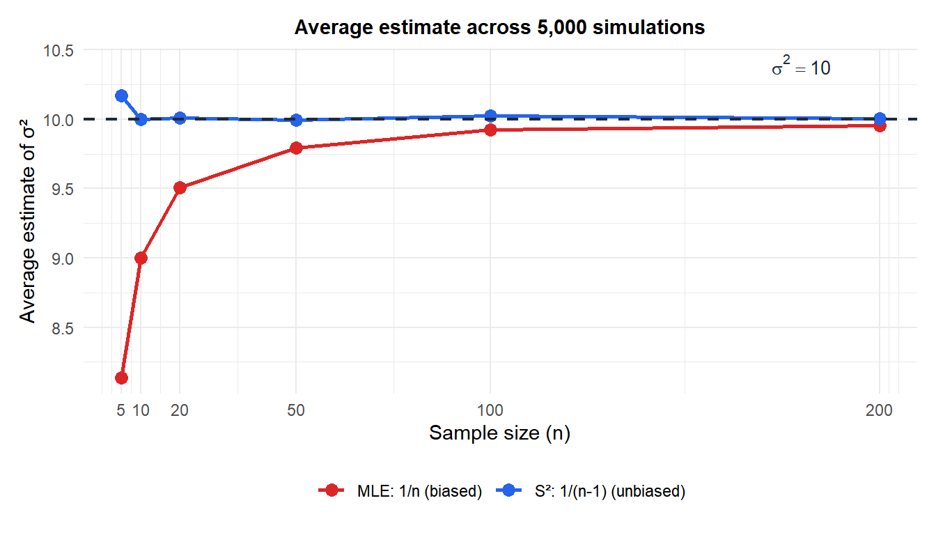
The simulation confirms: \(S^2\) (blue) stays on target at \(\sigma^2 = 10\) for all sample sizes, while the MLE (red) systematically underestimates, especially for small \(n\).
Step-by-step example
A quality engineer measures the diameter (in mm) of 8 ball bearings from a production run:
\[12.1,\; 11.9,\; 12.3,\; 12.0,\; 11.8,\; 12.2,\; 12.1,\; 12.4\]
Step 1: compute the sample mean:
\[\bar{x} = \frac{12.1 + 11.9 + \cdots + 12.4}{8} = \frac{96.8}{8} = 12.1 \text{ mm}\]
Step 2: compute squared deviations:
\[\sum(x_i - \bar{x})^2 = 0 + 0.04 + 0.04 + 0.01 + 0.09 + 0.01 + 0 + 0.09 = 0.28\]
Step 3: divide by \(n - 1 = 7\):
\[S^2 = \frac{0.28}{7} = 0.04 \text{ mm}^2, \qquad S = \sqrt{0.04} = 0.2 \text{ mm}\]
The estimated population variance is \(0.04\) mm², and the standard deviation is \(0.2\) mm. The MLE would give \(0.28/8 = 0.035\) mm², underestimating by 12.5%.
💡 Sample variance vs sample standard deviation
\(S^2\) is unbiased for \(\sigma^2\), but \(S = \sqrt{S^2}\) is not unbiased for \(\sigma\). The square root of an unbiased estimator is not itself unbiased (Jensen’s inequality for concave functions). In practice this bias is small and \(S\) is still the standard estimator for \(\sigma\), but technically a correction factor exists for normal populations.

