Estimation of a population mean
The sample mean \(\bar{X}\) is the standard point estimator for the population mean \(\mu\). Understanding its properties, its sampling distribution, and its standard error is the foundation of any inference about means.
The estimator: sample mean
Given a random sample \(x_1, x_2, \ldots, x_n\) from a population with mean \(\mu\) and variance \(\sigma^2\), the natural estimator for \(\mu\) is the sample mean:
\[\bar{X} = \frac{1}{n} \sum_{i=1}^{n} X_i\]
The sample mean has three key properties that make it the standard choice:
- Unbiased: \(E[\bar{X}] = \mu\). On average across all possible samples, \(\bar{X}\) hits the target.
- Consistent: as \(n\) increases, \(\bar{X}\) converges to \(\mu\).
- Efficient: among all unbiased estimators, \(\bar{X}\) has the smallest variance when the population is normal (it achieves the Cramér-Rao bound).
Sampling distribution of the mean
Before collecting data, \(\bar{X}\) is a random variable. Its distribution across all possible samples of size \(n\) is the sampling distribution of the mean:
\[\bar{X} \sim N\!\left(\mu,\ \frac{\sigma}{\sqrt{n}}\right) \quad \text{exactly, if the population is normal}\]
By the Central Limit Theorem (CLT), this approximation holds for any population with finite variance when \(n\) is large enough (typically \(n \geq 30\) is used as a rule of thumb, though the required \(n\) depends on the shape of the population).
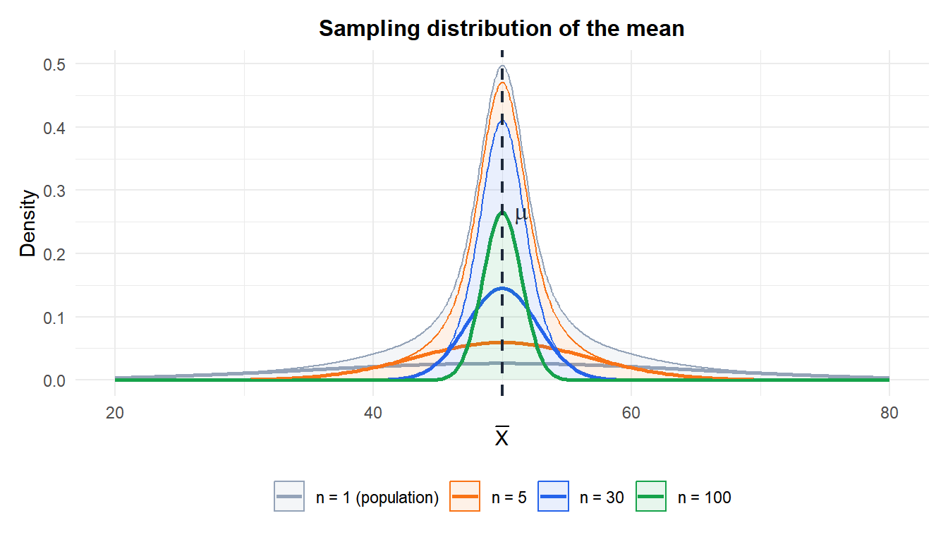
Figure 1: As n increases, the sampling distribution of the mean becomes narrower and more symmetric, regardless of the population distribution
Standard error of the mean
The spread of the sampling distribution is measured by the standard error (SE):
\[\text{SE}(\bar{X}) = \frac{\sigma}{\sqrt{n}}\]
The SE tells you how much \(\bar{X}\) is expected to vary from sample to sample. It decreases as \(n\) increases: doubling the sample size halves the standard error (you need four times the data to halve the SE).
In practice \(\sigma\) is unknown and is estimated by the sample standard deviation \(S\):
\[\widehat{\text{SE}}(\bar{X}) = \frac{S}{\sqrt{n}}\]
⚠️ Standard error is not the same as standard deviation
- Standard deviation (\(S\)): measures the spread of individual observations around the sample mean. It describes variability in the data.
- Standard error (\(\widehat{\text{SE}}\)): measures the spread of the sample mean across different samples. It describes the precision of the estimate.
A large dataset can have a large \(S\) (the data is spread out) and a very small \(\widehat{\text{SE}}\) (the mean is estimated precisely). They answer different questions.
Step-by-step example
A hospital records the length of stay (in days) for a random sample of 40 patients admitted with a specific diagnosis. The results are: \(\bar{x} = 6.4\) days, \(S = 3.1\) days.
Point estimate of the population mean:
\[\hat{\mu} = \bar{x} = 6.4 \text{ days}\]
Estimated standard error:
\[\widehat{\text{SE}} = \frac{S}{\sqrt{n}} = \frac{3.1}{\sqrt{40}} = \frac{3.1}{6.32} \approx 0.49 \text{ days}\]
Interpretation: the best single estimate of the average length of stay for all patients with this diagnosis is 6.4 days. The standard error of 0.49 days tells us that if we repeated this study many times, the sample mean would typically fall within about 0.49 days of the true mean.
Same population (\(\mu = 6.4\), \(S = 3.1\)), different sample sizes:
| \(n\) | \(\widehat{\text{SE}} = S/\sqrt{n}\) | Interpretation |
|---|---|---|
| 10 | \(3.1/\sqrt{10} \approx 0.98\) | Mean known to within ~1 day |
| 40 | \(3.1/\sqrt{40} \approx 0.49\) | Mean known to within ~0.5 days |
| 160 | \(3.1/\sqrt{160} \approx 0.25\) | Mean known to within ~0.25 days |
| 640 | \(3.1/\sqrt{640} \approx 0.12\) | Mean known to within ~0.12 days |
Each fourfold increase in \(n\) halves the standard error. Precision improves with more data, but with diminishing returns.
Why the sample mean works: the CLT
The Central Limit Theorem guarantees that \(\bar{X}\) is approximately normally distributed for large \(n\), regardless of the shape of the population. This is what makes the sample mean universally useful:
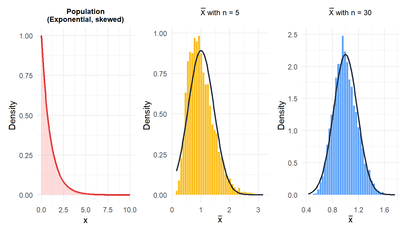
Figure 2: Means of samples from a heavily right-skewed exponential population converge to normality as n increases
Even starting from a heavily skewed exponential distribution, the sampling distribution of \(\bar{X}\) is already approximately normal by \(n = 30\).
💡 When to use z vs t for inference about the mean
The choice depends on what is known:
- \(\sigma\) known: use the standard normal \(Z = (\bar{X} - \mu)/(\sigma/\sqrt{n})\). Rare in practice.
- \(\sigma\) unknown, \(n\) large: the \(t\) distribution with \(n-1\) degrees of freedom. For \(n \geq 30\) it is nearly indistinguishable from the normal.
- \(\sigma\) unknown, \(n\) small: the \(t\) distribution is essential. It has heavier tails to account for the additional uncertainty from estimating \(\sigma\).
In practice: always use \(t\) when \(\sigma\) is unknown. For large \(n\), \(t\) and \(z\) give the same result anyway.

