Weighted mean
The arithmetic mean treats every observation as equally important. The weighted mean generalizes it by letting each value count in proportion to a weight \(w_i\), which matters whenever observations genuinely do not carry the same importance, size, or reliability.
The formula
The weighted mean replaces the plain sum in the arithmetic mean with a weighted sum, and divides by the sum of the weights instead of the count:
\[\bar{x}_w = \frac{\sum_{i=1}^n w_i x_i}{\sum_{i=1}^n w_i}\]
The ordinary arithmetic mean is the special case where every \(w_i\) is equal: the weights cancel out of the formula entirely, leaving the plain average. The weights do not need to sum to 1 or to 100, since the formula divides by their total, only their relative sizes matter.
Worked example: a weighted portfolio return
Sizes that differ this much are exactly where the weighted and unweighted mean part ways the most.
An investor holds four positions. Each has its own return for the year, but the positions are far from equally sized, so a plain average of the four returns would misrepresent how the portfolio actually performed.
| Investment | Amount invested | Return |
|---|---|---|
| A | $10,000 | 8% |
| B | $25,000 | -3% |
| C | $5,000 | 15% |
| D | $60,000 | 5% |
Weighting each return by the dollar amount behind it:
\[\bar{x}_w = \frac{10000(8) + 25000(-3) + 5000(15) + 60000(5)}{10000+25000+5000+60000} = \frac{380000}{100000} = 3.8\%\]
The plain, unweighted mean of the four returns is \((8 - 3 + 15 + 5)/4 = 6.25\%\), noticeably higher. The unweighted figure is pulled up by the 15% return on the smallest position ($5,000) and ignores that the single biggest drag, the -3% return, sits on the second-largest position ($25,000). The weighted mean of 3.8% is the number that actually describes what happened to the investor’s money.

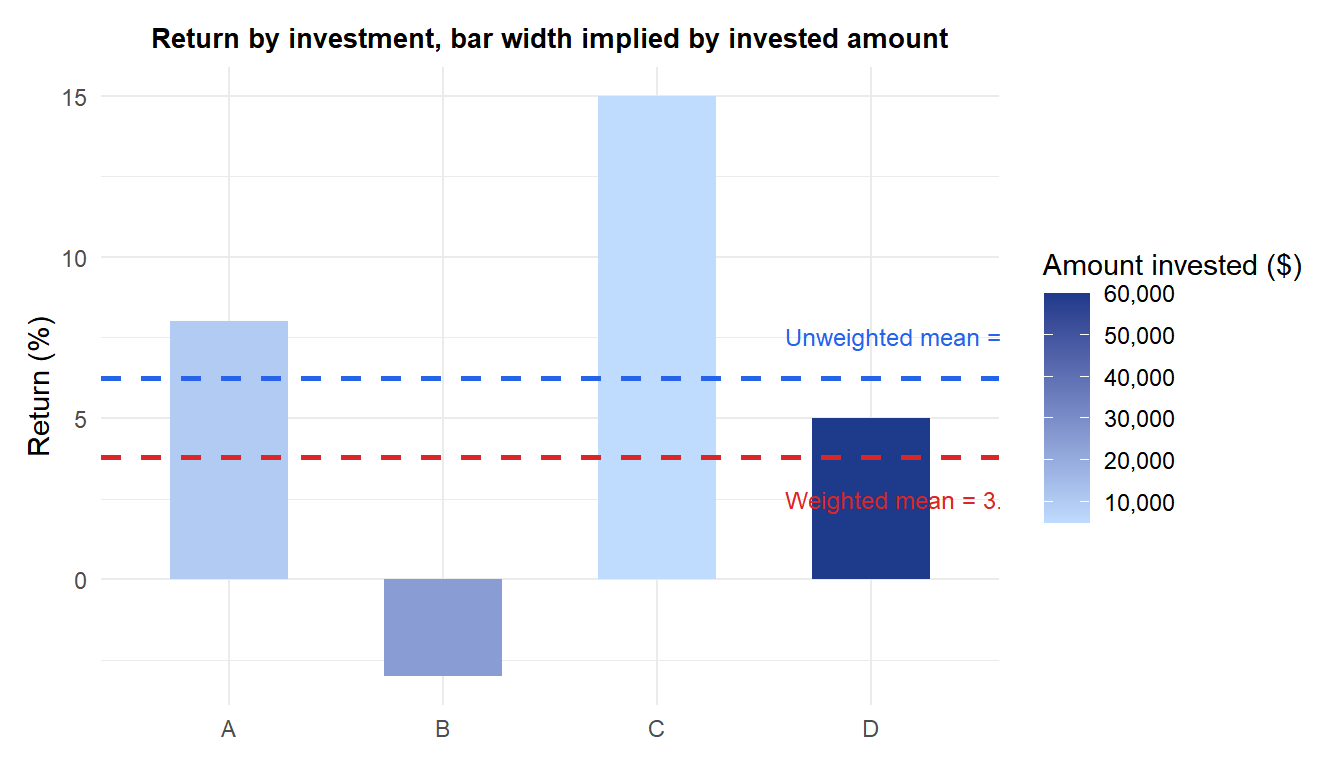
The bar fill shows how much money sits behind each return. The weighted mean (red) sits well below the unweighted mean (blue), pulled down by the large, negative-return position B, exactly the position a naive unweighted average would under-count.
Why ignoring the weights is a real mistake
Treating unequal-sized groups as if they were equal-sized is not a harmless simplification, it can flip the practical conclusion entirely.
⚠️ Averaging rates across groups of different sizes
Suppose three regions report unemployment rates of 4%, 9% and 12%, with populations of 2,000,000, 500,000 and 100,000 respectively. The naive, unweighted average of the three rates is \((4+9+12)/3 = 8.33\%\). The population-weighted national rate is \(5.27\%\), nearly 3 points lower, because the unweighted average silently gives the smallest region (100,000 people) the same influence as the largest region (2,000,000 people), twenty times its actual share. Whenever you average a rate, a percentage, or a ratio across groups, ask what the groups’ sizes were and whether a plain average is secretly treating them as equal.
Running it in R
R’s weighted.mean() takes the values and the weights directly, no need to implement the formula by hand:
amount <- c(10000, 25000, 5000, 60000)
ret    <- c(8, -3, 15, 5)

weighted.mean(ret, amount)   # 3.8, weighted by dollar amount
mean(ret)                    # 6.25, plain unweighted mean
💡 Where weighted means show up in practice
Beyond portfolio returns, weighted means are everywhere once you look for them: consumer price indices average price changes across goods weighted by how much of each a typical household buys; grade point averages weight course grades by credit hours; survey statisticians apply weights to correct for groups that responded less often than their true share of the population; and variance itself has a weighted version, used whenever the underlying observations are group averages of different sample sizes rather than raw individual measurements.