Calculate the mean in statistics
The mean is the most widely used measure of central tendency, but it comes in several forms. This tutorial covers the arithmetic, weighted, truncated and geometric mean: what each one measures, when to use it, and when to avoid it.
Arithmetic mean
The arithmetic mean is what most people mean when they say “average.” It is defined as the sum of all values divided by the number of values.
For a set of \(n\) values \((x_1, x_2, \dots, x_n)\), the mean \(\bar{x}\) is:
\[\bar{x} = \frac{\sum_{i = 1}^n x_i}{n},\]
being \(x_i\) the observation \(i\) of \(x\).
Properties
The arithmetic mean has three properties that are useful when working with transformed data:
- Zero deviation sum: the sum of deviations from the mean is always zero, \(\sum_{i=1}^n (x_i - \bar{x}) = 0\).
- Translation: adding a constant \(c\) to every value shifts the mean by the same amount. If \(Y = X + c\), then \(\bar{y} = \bar{x} + c\).
- Scale: multiplying every value by a constant \(c\) multiplies the mean by that constant. If \(Y = cX\), then \(\bar{y} = c\bar{x}\).
- Linear transformation: combining both, if \(Y = aX + b\), then \(\bar{y} = a\bar{x} + b\).
The selling prices of four cars are: 25,000, 32,000, 15,000 and 72,000 USD.
Mean price:
\[\bar{x} = \frac{25000 + 32000 + 15000 + 72000}{4} = 36{,}000 \text{ USD.}\]
If every price increases by 5,000 USD, what is the new mean?
By the translation property: \(\bar{y} = 36{,}000 + 5{,}000 = 41{,}000\) USD. No need to recalculate from scratch.
If every price increases by 10%, what is the new mean?
By the scale property: \(\bar{y} = 36{,}000 \times 1.1 = 39{,}600\) USD.
The outlier problem
The arithmetic mean is sensitive to extreme values. A single outlier can pull the mean far from where most of the data sits.
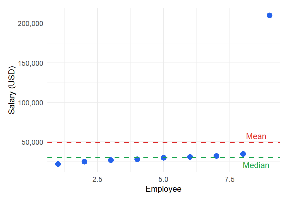
Figure 1: One outlier shifts the mean significantly, while the median stays stable
⚠️ When not to use the arithmetic mean
Avoid the arithmetic mean when:
- The data has heavy outliers: one CEO’s salary in a sample of workers will make the mean useless as a “typical” value.
- The distribution is strongly skewed: house prices, income, and city populations are classic examples. The median is a better choice.
- The variable is ordinal: averaging satisfaction scores (1 = poor, 5 = excellent) assumes equal distances between categories, which is not guaranteed.
Truncated mean
The truncated mean removes a fixed percentage of the lowest and highest values before calculating the mean. It is a simple way to reduce the influence of outliers without switching to a completely different measure.
To compute the truncated mean at \(p\)%: sort the data, remove the \(p\)% of values from each end, and calculate the arithmetic mean of what remains.
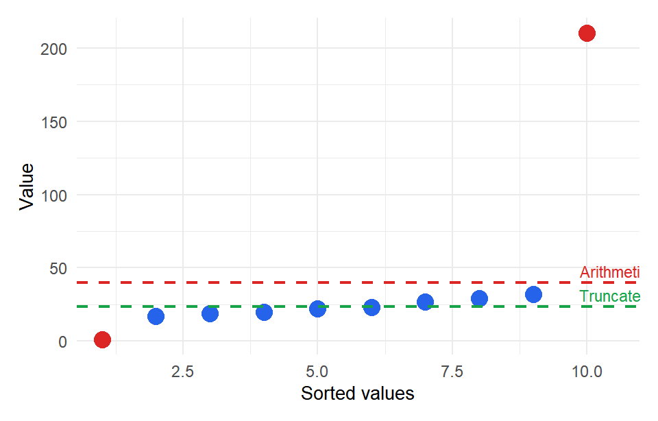
Figure 2: Truncated mean at 10%: the two extreme values (red) are removed before averaging
Consider the following 10 values: (1, 17, 19, 20, 22, 23, 27, 29, 32, 210).
The arithmetic mean is: \[\bar{x} = \frac{1 + 17 + \cdots + 210}{10} = 40.\]
At 10% truncation, we remove 1 value from each end (10% of 10). Sorting and removing the extremes:
1, 17, 19, 20, 22, 23, 27, 29, 32, 210
The truncated mean is: \[\bar{x}_t = \frac{17 + 19 + 20 + 22 + 23 + 27 + 29 + 32}{8} = 23.625.\]
The two outliers (1 and 210) were pulling the arithmetic mean up to 40, far from where most values actually are.
💡 Real-world use of the truncated mean
Weighted mean
The arithmetic mean assumes every observation has the same importance. The weighted mean allows different values to contribute differently, according to a weight \(w_i\) assigned to each observation \(x_i\):
\[\bar{x}_w = \frac{\sum_{i=1}^k x_i \cdot w_i}{\sum_{i=1}^k w_i}.\]
A course has three assessments with different weights: a midterm (20%), a project (20%) and a final exam (60%). A student scores 5, 7 and 8.
\[\bar{x}_w = \frac{5 \cdot 0.2 + 7 \cdot 0.2 + 8 \cdot 0.6}{0.2 + 0.2 + 0.6} = \frac{1 + 1.4 + 4.8}{1} = 7.2.\]
With a simple arithmetic mean the score would be 6.67. The weighted mean reflects the fact that the final exam matters more.
⚠️ The weights must sum to a meaningful total
The formula divides by (\sum w_i), so the weights do not need to sum to 1 or 100. However, make sure the weights reflect actual relative importance. A common mistake is using counts as weights when what you want is proportional weights, or vice versa.
Geometric mean
The geometric mean is the appropriate average when working with values that are multiplied together, such as growth rates, ratios, or indices. It is defined as the \(k\)-th root of the product of \(k\) values:
\[\bar{x}_g = \left(\prod_{i=1}^k x_i\right)^{\frac{1}{k}}.\]
An equivalent and often more practical formula uses logarithms:
\[\bar{x}_g = \exp\left(\frac{1}{k} \sum_{i=1}^k \ln(x_i)\right).\]
An investment grows by 5%, 10% and 20% in three consecutive years. What is the average annual growth rate?
Convert to multipliers: \(x = (1.05,\ 1.10,\ 1.20)\).
\[\bar{x}_g = (1.05 \times 1.10 \times 1.20)^{1/3} = 1.386^{1/3} \approx 1.1154.\]
The average annual growth rate is approximately 11.54%.
To verify: \(1.05 \times 1.10 \times 1.20 = 1.386\), and \(1.1154^3 \approx 1.386\). Correct.
Using the arithmetic mean instead would give \((1.05 + 1.10 + 1.20)/3 = 1.1167\), or 11.67%. The arithmetic mean slightly overestimates compound growth.
⚠️ Geometric mean requires all positive values
The geometric mean is only defined when all values are positive. If any value is zero or negative, the formula breaks down. For growth rates, make sure you are working with multipliers (e.g. 1.05 for 5% growth), not raw percentages.

