Quantiles in statistics
Quantiles divide a sorted dataset into equal parts. They tell you not just where the center is, but how the data is spread across the full range. Quartiles, deciles, and percentiles are all quantiles, just with different numbers of divisions.
Definition
A quantile of order \(p\) (where \(0 < p < 1\)) is the value \(q_p\) that divides the sorted data so that at least a fraction \(p\) of the observations fall at or below it, and at least a fraction \(1-p\) fall at or above it.
In plain terms: the quantile \(q_p\) is the value below which \(p \times 100\%\) of the data lies.
The three most common families of quantiles are:
- Quartiles: divide the data into 4 equal parts (3 cut points).
- Deciles: divide the data into 10 equal parts (9 cut points).
- Percentiles: divide the data into 100 equal parts (99 cut points).
These are not different concepts, they are the same idea applied at different resolutions. The 25th percentile is the same as the first quartile \(Q_1\). The 50th percentile is the same as the second quartile \(Q_2\) and the median.
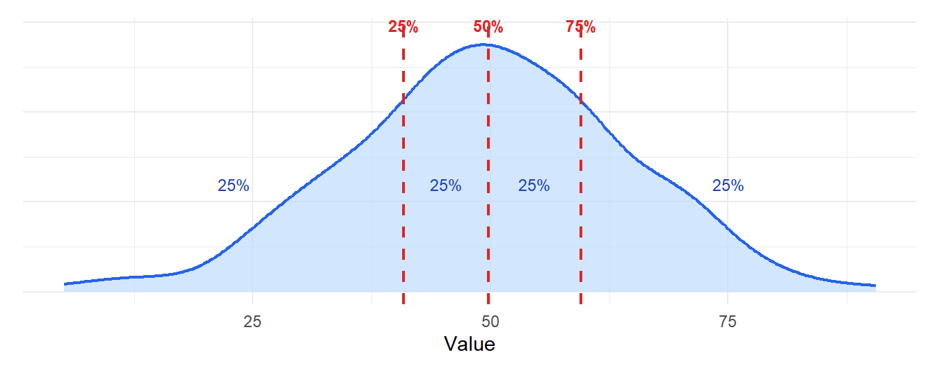
Figure 1: Quartiles divide the distribution into four equal parts
Quartiles
Quartiles are the three values \(Q_1\), \(Q_2\) and \(Q_3\) that split the sorted data into four parts of equal size.
- \(Q_1\) (first quartile, 25th percentile): 25% of the data falls below this value.
- \(Q_2\) (second quartile, 50th percentile): this is the median.
- \(Q_3\) (third quartile, 75th percentile): 75% of the data falls below this value.
The difference \(Q_3 - Q_1\) is called the interquartile range (IQR). It measures the spread of the central 50% of the data and is one of the most robust measures of dispersion.
Given the dataset: (3, 7, 8, 5, 12, 14, 21, 13, 18)
Sort the data: \((3, 5, 7, 8, 12, 13, 14, 18, 21)\)
- \(Q_2\) is the median of the full dataset: \(Q_2 = 12\)
- \(Q_1\) is the median of the lower half \((3, 5, 7, 8)\): \(Q_1 = \frac{5+7}{2} = 6\)
- \(Q_3\) is the median of the upper half \((13, 14, 18, 21)\): \(Q_3 = \frac{14+18}{2} = 16\)
- \(IQR = Q_3 - Q_1 = 16 - 6 = 10\)

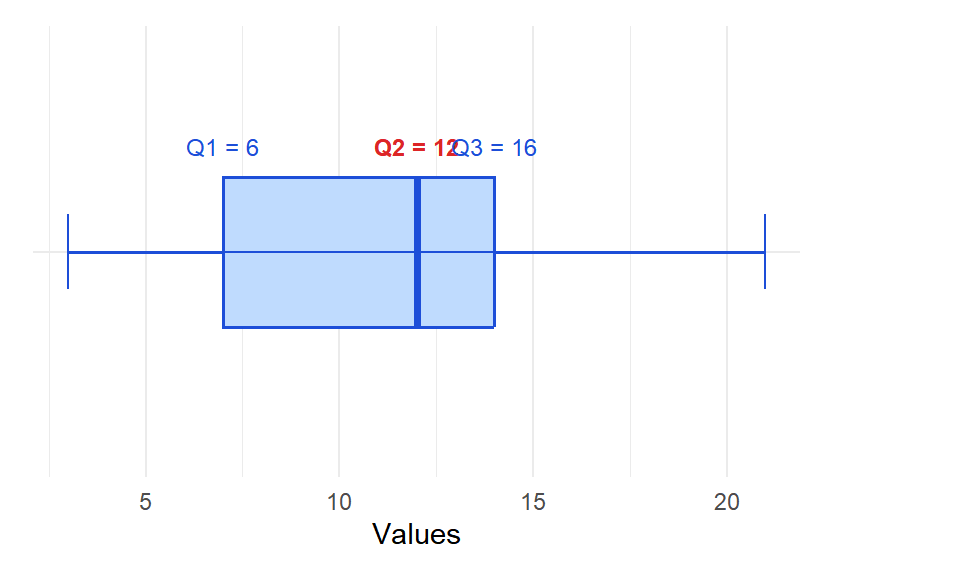
Figure 2: A boxplot visualizes the quartiles: the box spans Q1 to Q3, the line inside is Q2
💡 Quartiles and the boxplot
Deciles
Deciles are the 9 values \(d_1, d_2, \dots, d_9\) that divide the sorted data into 10 equal parts. Each decile corresponds to a multiple of 10% of the distribution.
Note that \(d_5 = Q_2 = Me\): the fifth decile, second quartile, and median are all the same value.
A class of 30 students takes an exam. The scores sorted in order range from 41 to 98. The deciles split this range into 10 bands of equal frequency (3 students each):
- \(d_1 = 48\): 10% of students scored below 48.
- \(d_3 = 61\): 30% scored below 61.
- \(d_5 = 72\): half the class scored below 72 (this is also the median).
- \(d_9 = 94\): 90% scored below 94, so only 3 students are in the top 10%.
A student who scored 72 is exactly at the median. A student who scored 94 is in the top decile.
Percentiles
Percentiles divide the data into 100 equal parts. The \(k\)-th percentile \(p_k\) is the value below which \(k\%\) of the observations fall.
Percentiles are the most granular of the three families and are widely used when comparing an individual’s position within a reference population.
When a doctor measures a child’s height and weight, the result is reported as a percentile relative to a reference population of children the same age and sex:
- A child at the 50th percentile for height is taller than exactly half of children the same age.
- A child at the 97th percentile is taller than 97% of peers, which may warrant further evaluation.
- A child below the 3rd percentile is shorter than 97% of peers.
The cutoffs of 3rd and 97th percentile are standard clinical thresholds precisely because they are easy to interpret: they represent the extreme 3% at each end of the distribution.
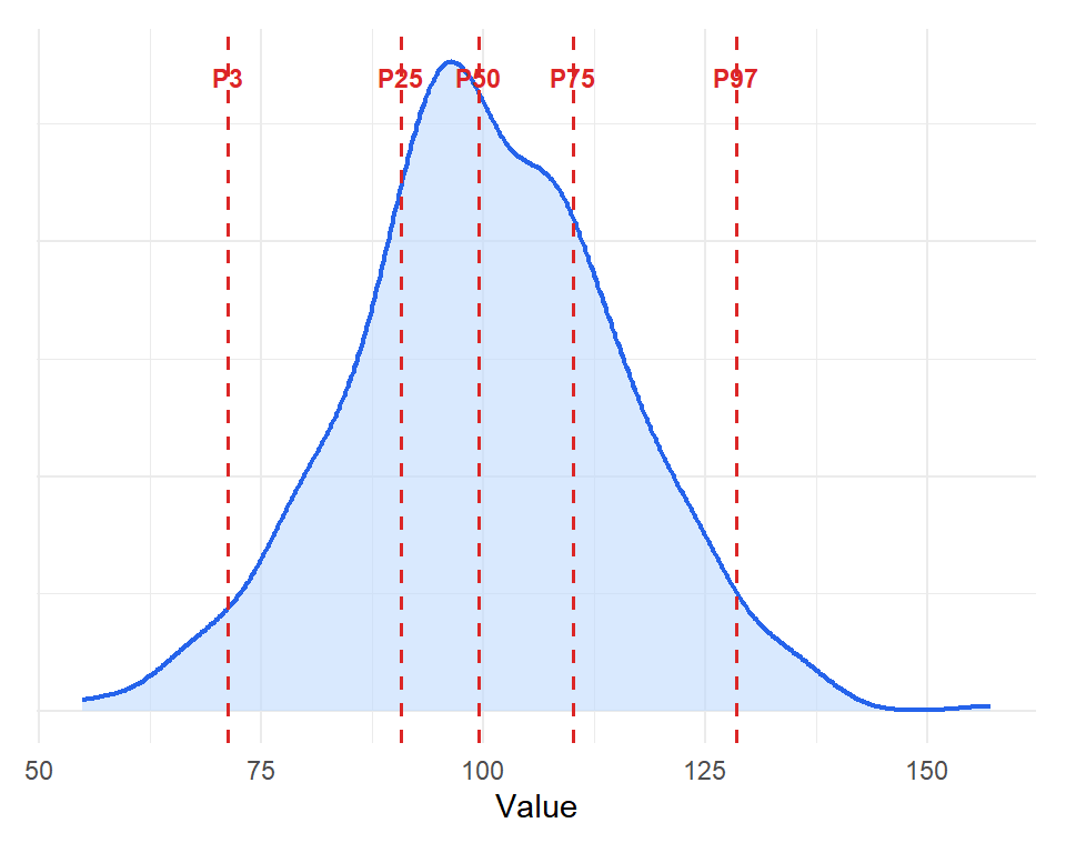
Figure 3: Percentile bands: each band contains 1% of the data
How to calculate quantiles
The general formula for the position of the \(k\)-th quantile in a sorted dataset of size \(n\), with \(m\) total parts, is:
\[q_k = \frac{k(n+1)}{m}\]
If the result is an integer \(i\), the quantile is \(x_i\). If it falls between two positions \(i\) and \(i+1\), interpolate:
\[q_k = x_i + (pos - i)(x_{i+1} - x_i)\]
Dataset: (55, 60, 65, 70, 75, 80, 85, 90, 95, 100) ((n = 10), already sorted).
Position of \(Q_1\) (\(k=1\), \(m=4\)): \[pos = \frac{1 \times (10+1)}{4} = 2.75\]
The position falls between the 2nd value (60) and the 3rd value (65). Interpolating: \[Q_1 = 60 + 0.75 \times (65 - 60) = 60 + 3.75 = 63.75\]
⚠️ There is no single formula for quantiles
Different software uses different interpolation methods. R alone has 9 different algorithms for computing quantiles (type 1 through type 9 in the quantile() function). This is why the quartile values you calculate by hand may not exactly match what R or Excel gives you. The differences are small for large datasets but can be noticeable with small samples.
Quick reference
| Name | Divisions | Cut points | Key relationships |
|---|---|---|---|
| Quartiles | 4 | \(Q_1, Q_2, Q_3\) | \(Q_2 = d_5 = p_{50} = Me\) |
| Deciles | 10 | \(d_1, \dots, d_9\) | \(d_5 = Q_2 = Me\) |
| Percentiles | 100 | \(p_1, \dots, p_{99}\) | \(p_{25} = Q_1\), \(p_{50} = Me\), \(p_{75} = Q_3\) |

