Calculate the median in statistics
The median is the value that splits a sorted dataset exactly in half. It is more robust than the mean when data contains outliers or is strongly skewed, which makes it the preferred measure in fields like real estate, income analysis, and medicine.
Definition
The median is the central value of a sorted dataset: half the observations fall below it and half above it. It is represented as \(Me\).
The formula depends on whether the sample size \(n\) is odd or even:
\[ Me(x) = \begin{cases} x_{(n+1)/2} &\text{if n is odd} \\\ \\\ \frac{x_{(n/2)} + x_{((n/2) + 1)}}{2} &\text{if n is even,} \end{cases} \]
being \(x\) an ordered vector of values in increasing order of size \(n\).
The key step that many students miss: you must sort the data first. The median is always a positional measure, it depends on where a value sits in the ordered sequence, not on its magnitude.
⚠️ Sort before you calculate
A very common mistake is picking the middle element of the original unsorted data. For example, in (x = (83, 133, 104, 52, 57)) the middle element is 104, but the median of the sorted sequence ((52, 57, 83, 104, 133)) is 83. Always sort first.
Properties
- Linear transformation: if \(Y = aX + b\), then \(Me(Y) = a \cdot Me(X) + b\).
- Robustness: the median is not affected by outliers. Adding an extreme value does not change its position in the sorted sequence.
- Variable types: the median applies to quantitative variables and to qualitative ordinal variables (where a natural order exists).
- Splits the distribution at 50%: by definition, the median is the 50th percentile, also written \(Q_2\).
Examples
Odd sample size
Consider the following data: \[x = (83, 133, 104, 52, 57, 53, 126, 115, 105, 100, 67).\]
The sample size is \(n = 11\) (odd), so the median is the value at position \((11+1)/2 = 6\) in the sorted sequence.
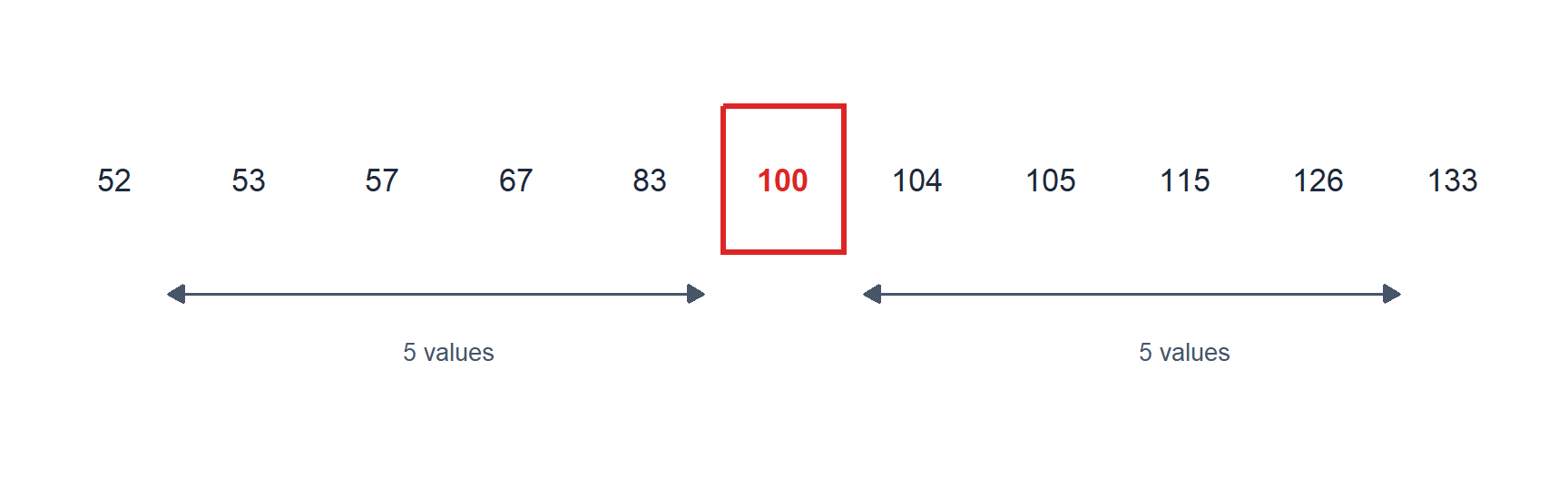
Figure 1: Sorted data: the median (red box) leaves 5 values on each side
The median is \(Me(x) = 100\).
Even sample size
Now remove the value 100 from the previous dataset: \[x = (83, 133, 104, 52, 57, 53, 126, 115, 105, 67).\]
The sample size is now \(n = 10\) (even), so the median is the mean of the values at positions \(n/2 = 5\) and \(n/2 + 1 = 6\) in the sorted sequence.
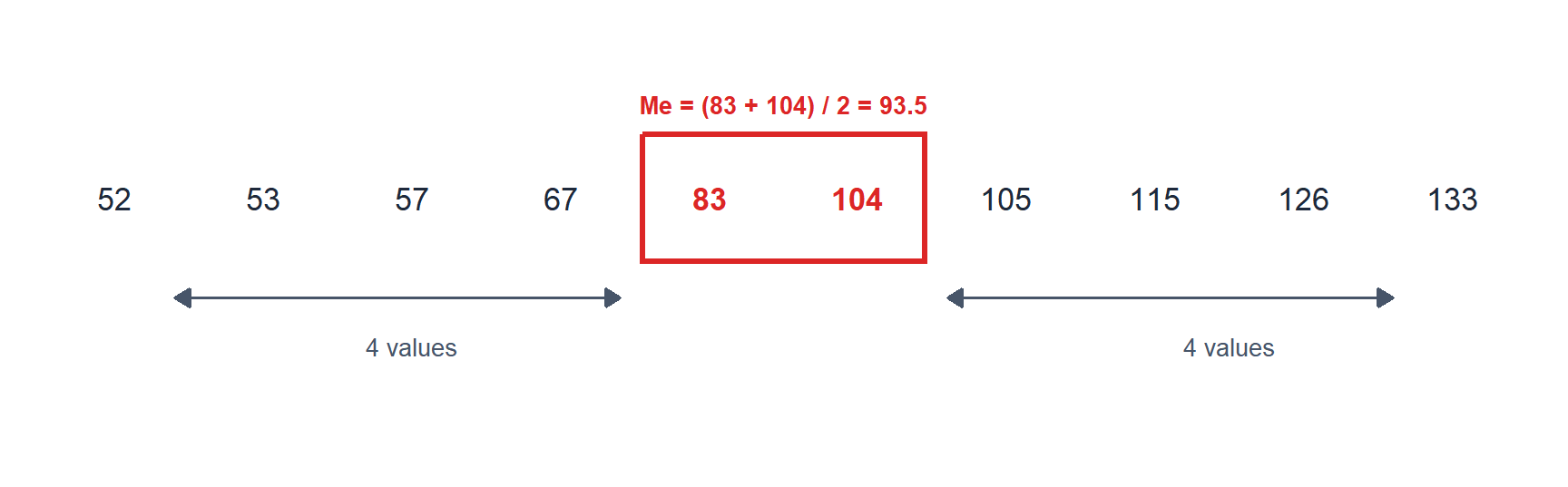
Figure 2: Even sample size: the median is the average of the two central values (red box)
The median is \(Me(x) = \frac{83 + 104}{2} = 93.5\).
Mean vs. median: when to use each
The mean and median both measure the center of a distribution, but they behave very differently when data is skewed or contains outliers.
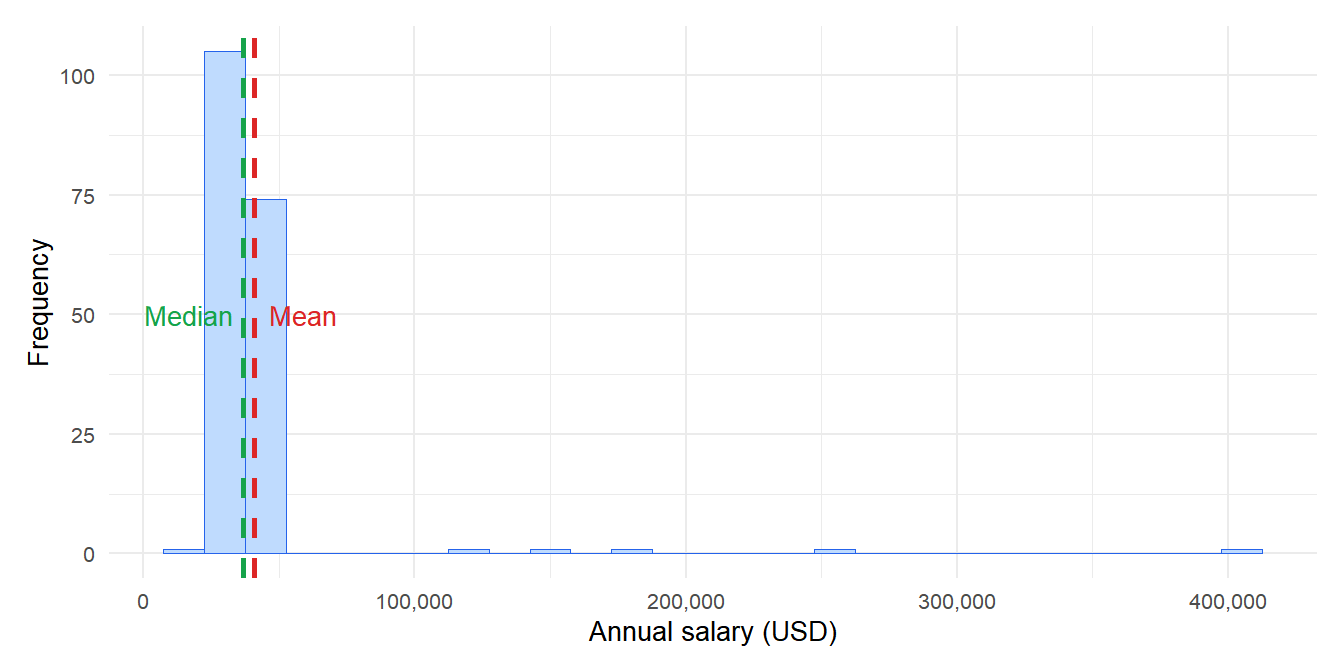
Figure 3: Skewed distribution: the mean is pulled toward the tail, the median stays near the bulk of the data
- Salaries: a few executives with very high salaries pull the mean far above what most employees earn. The median salary is the more honest description of a “typical” worker’s pay.
- House prices: a handful of luxury properties distort the mean. Real estate reports always quote the median price.
- Response times: a small number of very slow server requests (timeouts, errors) inflate the mean. The median gives a better picture of typical performance.
⚠️ The median ignores the magnitude of values
The median only cares about order, not about how far apart the values are. In the dataset ((1, 2, 3, 4, 100)) and in ((1, 2, 3, 4, 5)), the median is 3 in both cases. If the actual size of the values matters for your analysis, the mean captures that information and the median does not.
💡 A quick rule of thumb

