What is a time series?
A time series is a sequence of observations indexed by time. Unlike cross-sectional data, consecutive observations in a time series are typically correlated: today’s value depends on yesterday’s. This dependence structure is what makes time series both more informative and more challenging to analyze than independent data.
Definition
A time series is a set of observations \(\{y_t\}\) where \(t\) indexes time: \(t = 1, 2, \ldots, T\). The observations may be recorded at any regular frequency: annually, quarterly, monthly, weekly, daily, or intraday.
Examples across domains:
- Economics: monthly GDP, quarterly inflation, daily stock prices.
- Meteorology: daily temperature, hourly wind speed, annual rainfall.
- Business: weekly sales, monthly website traffic, daily energy consumption.
- Medicine: heart rate over time, daily patient admissions, weekly disease incidence.
The fundamental challenge: observations are not independent. Standard statistical methods (regression, hypothesis tests, confidence intervals) assume i.i.d. data. Applying them directly to time series produces incorrect standard errors and misleading inferences.
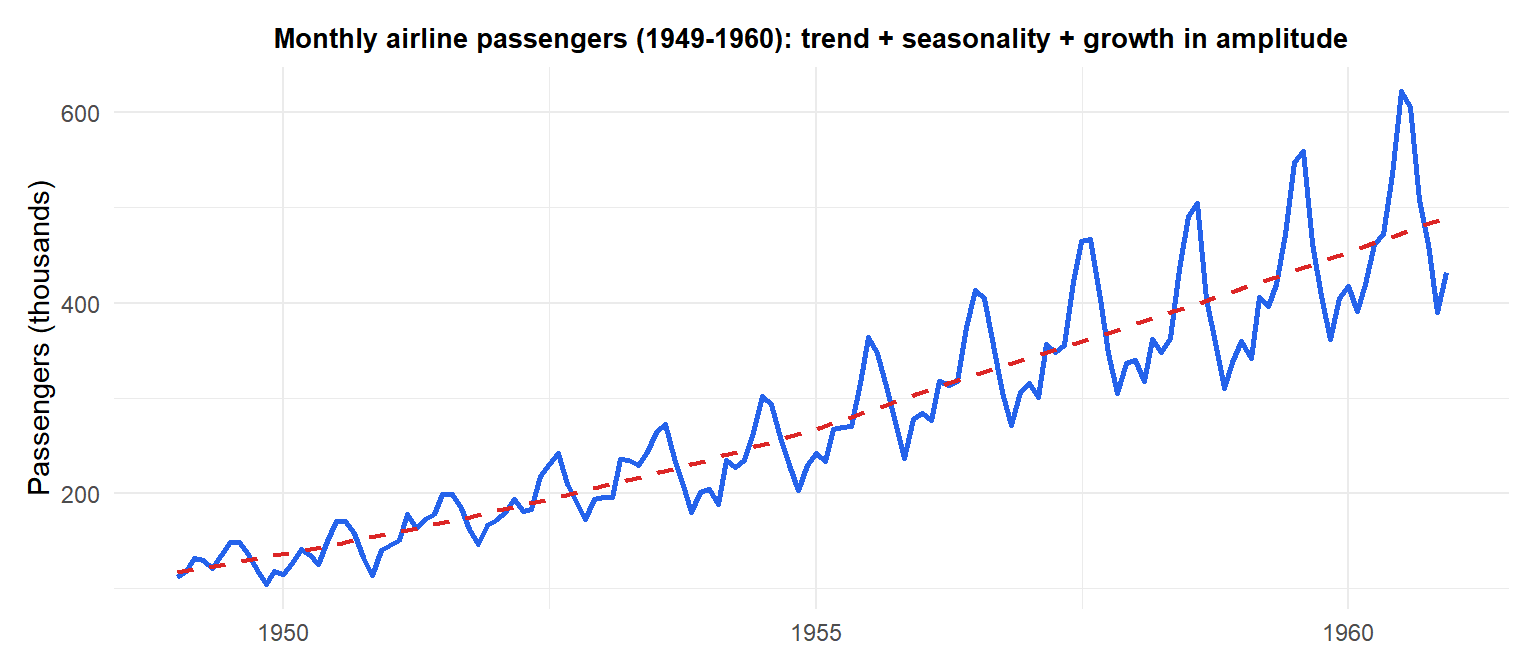
The airline series shows three features simultaneously: an upward trend (red dashed), a clear seasonal pattern (peaks in summer), and increasing amplitude over time (the seasonal swings grow with the level). These three features define the main components of a time series.
Components of a time series
Any time series can be thought of as a combination of four components:
- Trend (\(T_t\))
The long-term direction of the series: upward, downward, or flat. It reflects slow-moving forces: population growth, technological change, long-term economic cycles. The trend is usually smooth and persistent.
- Seasonality (\(S_t\))
Regular, repeating patterns at a fixed known frequency: daily (more traffic at rush hour), weekly (fewer hospital admissions on weekends), monthly (higher retail sales in December), quarterly. Seasonality has a fixed period and is predictable.
- Cycle (\(C_t\))
Longer-term oscillations that are not of fixed period: business cycles lasting several years, commodity price cycles. Unlike seasonality, cycles are irregular in timing and amplitude and harder to predict.
- Irregular component / noise (\(\varepsilon_t\))
The residual variation that cannot be attributed to trend, seasonality, or cycle. Ideally it is white noise: zero mean, constant variance, no autocorrelation.
Additive vs multiplicative decomposition
The four components combine either additively or multiplicatively:
\[y_t = T_t + S_t + C_t + \varepsilon_t \quad \text{(additive)}\]
\[y_t = T_t \times S_t \times C_t \times \varepsilon_t \quad \text{(multiplicative)}\]
Additive: seasonal fluctuations are constant in absolute terms regardless of the level. Use when the amplitude of seasonal swings does not change over time.
Multiplicative: seasonal fluctuations grow proportionally with the level. Use when the amplitude increases as the series grows (as in the airline data). Equivalent to applying an additive model to \(\log(y_t)\).
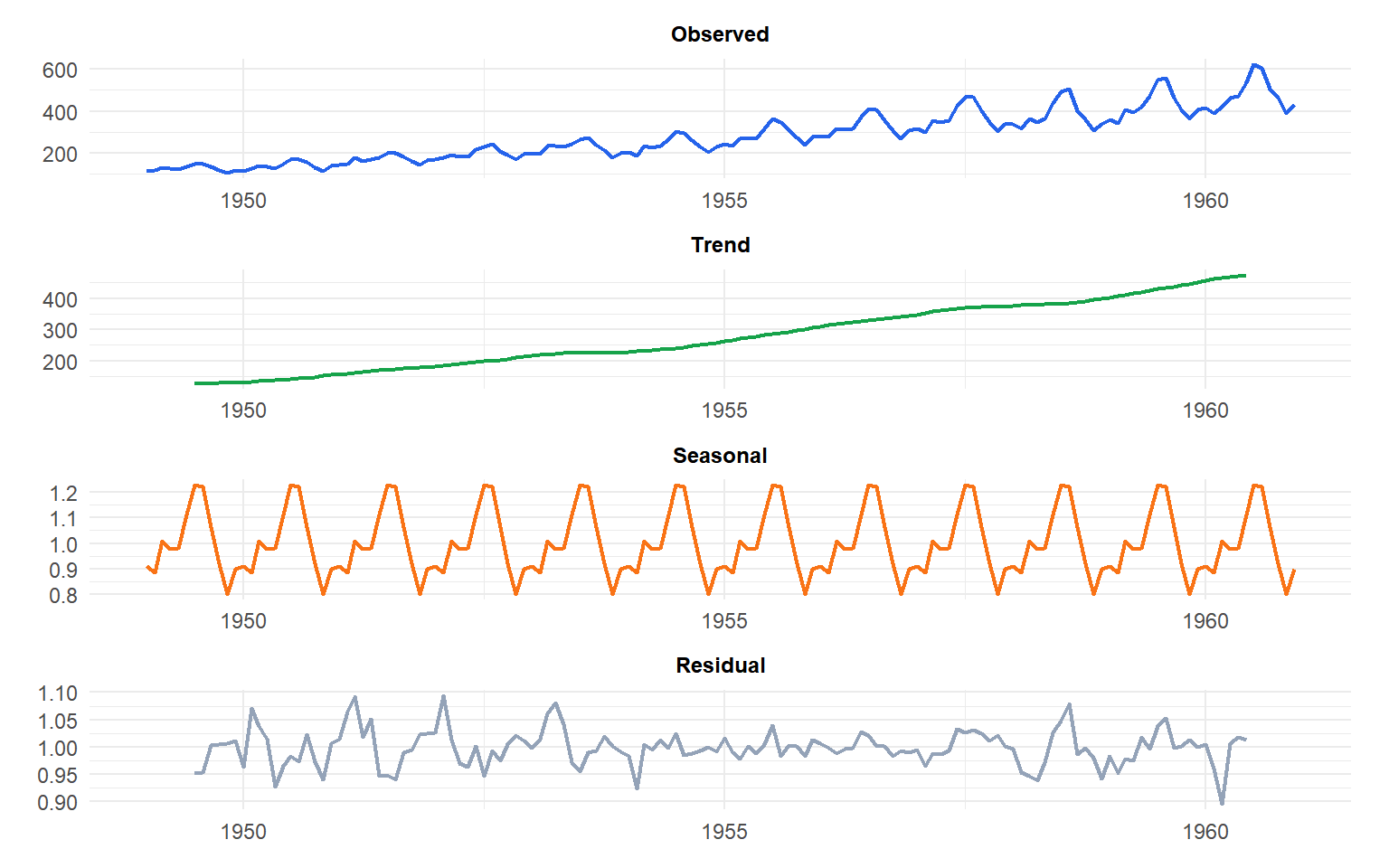
The multiplicative decomposition separates the airline series into its three components. The trend (green) shows steady growth. The seasonal component (orange) is stable in relative terms. The residual (grey) is approximately white noise, confirming that the decomposition has captured the main structure.
Stationarity
A time series is stationary if its statistical properties do not change over time:
\[E[y_t] = \mu \quad \forall t \qquad \text{(constant mean)}\] \[\text{Var}(y_t) = \sigma^2 \quad \forall t \qquad \text{(constant variance)}\] \[\text{Cov}(y_t, y_{t+k}) \text{ depends only on } k, \text{ not on } t \qquad \text{(constant autocovariance)}\]
Most time series models (AR, MA, ARMA, ARIMA) require or assume stationarity. A series with trend or growing variance is non-stationary and must be transformed before modelling.
Common transformations to achieve stationarity:
- Differencing: \(\Delta y_t = y_t - y_{t-1}\) removes a linear trend.
- Log transformation: \(\log(y_t)\) stabilizes variance that grows with the level.
- Seasonal differencing: \(y_t - y_{t-s}\) removes seasonal patterns.
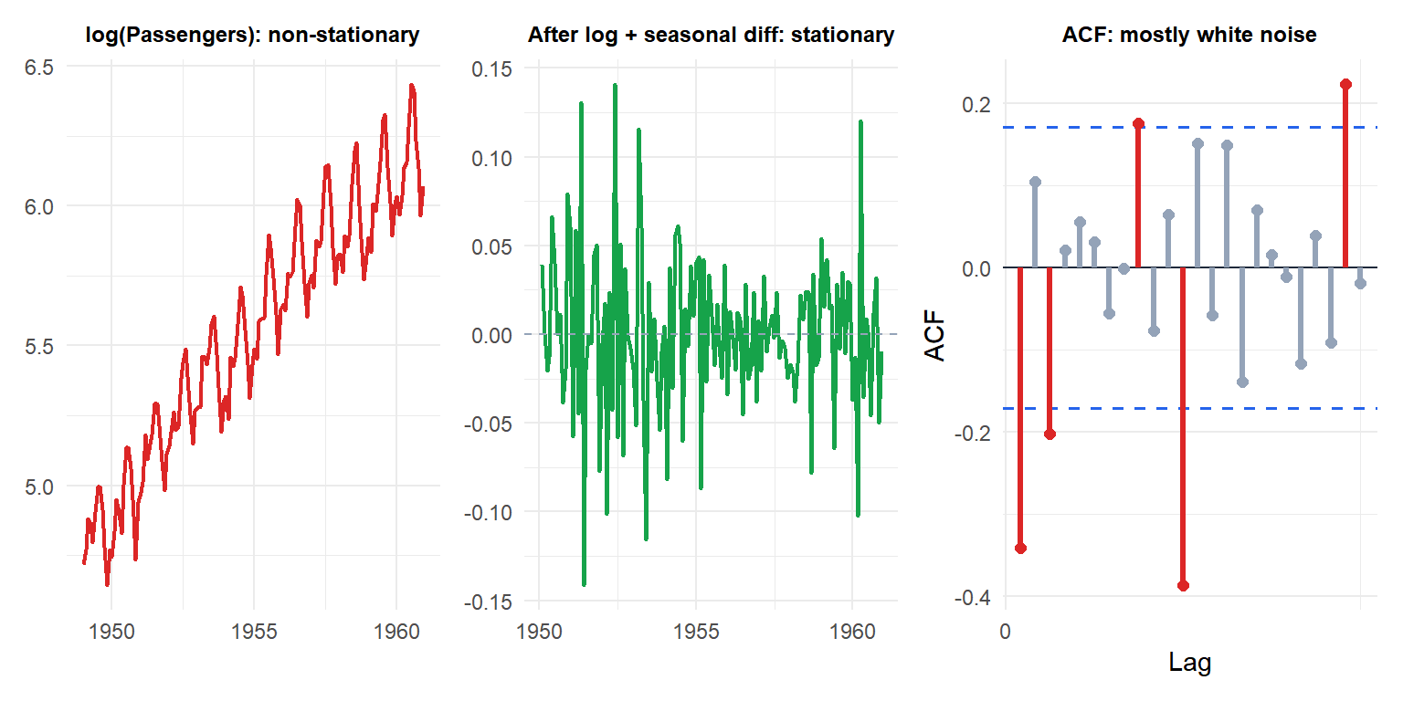
After log-transforming and applying seasonal differencing, the series becomes stationary: constant mean around zero, no visible trend, and an ACF with few significant spikes.
⚠️ Applying standard regression to non-stationary series produces spurious results
Regressing one non-stationary series on another can yield high \(R^2\) and significant coefficients even when the series are completely unrelated. This is spurious regression, a well-known pitfall first described by Granger and Newbold (1974).
Two non-stationary series that happen to trend together will appear correlated even if they have nothing in common. Always check for stationarity before modeling, and difference or transform the series if necessary.
Notation and lag operator
The lag operator \(L\) (or backshift operator \(B\)) is standard notation in time series:
\[Ly_t = y_{t-1}, \qquad L^k y_t = y_{t-k}\]
\[\Delta y_t = y_t - y_{t-1} = (1-L)y_t\]
\[\Delta^d y_t = (1-L)^d y_t \quad \text{($d$-th order differencing)}\]
This compact notation simplifies writing AR, MA, ARIMA and seasonal models.
Overview of time series models
The following posts cover the main modelling approaches:
| Model | Key idea | Best for |
|---|---|---|
| AR(\(p\)) | Current value depends on \(p\) past values | Short memory, mean-reverting series |
| MA(\(q\)) | Current value depends on \(q\) past errors | Series with sudden shocks that fade |
| ARMA(\(p,q\)) | Combines AR and MA | Stationary series |
| ARIMA(\(p,d,q\)) | ARMA after \(d\) differences | Non-stationary series with trend |
| SARIMA | ARIMA with seasonal terms | Seasonal series |
| Exponential smoothing | Weighted average of past values | Short-term forecasting |
| Holt-Winters | Trend + seasonal exponential smoothing | Series with trend and seasonality |
| ARIMAX | ARIMA with external regressors | Series driven by external factors |
| Kalman filter | State space representation | Noisy observations, dynamic systems |
💡 The modelling workflow for a time series
A standard approach:
- Plot the series: identify trend, seasonality, outliers.
- Transform if needed: log for variance stabilization, differencing for trend.
- Check stationarity: ADF or KPSS test.
- Examine ACF and PACF: identify candidate AR and MA orders.
- Fit candidate models: compare by AIC, BIC.
- Check residuals: they should be white noise (Ljung-Box test, ACF of residuals).
- Forecast and evaluate: use held-out data or cross-validation.

