SARIMA model
SARIMA extends ARIMA with seasonal AR, differencing and MA operators that capture patterns repeating every \(s\) periods. It is the standard model for monthly, quarterly or daily data with regular seasonal cycles such as retail sales, energy demand, or tourism.
Definition
A SARIMA(\(p,d,q\))(\(P,D,Q\))\(_s\) model is written compactly as:
\[\Phi_P(L^s)\,\phi_p(L)\,(1-L^s)^D(1-L)^d\,y_t = \Theta_Q(L^s)\,\theta_q(L)\,\varepsilon_t\]
where:
- \((p,d,q)\): non-seasonal AR order, differencing, MA order.
- \((P,D,Q)\): seasonal AR order, seasonal differencing, seasonal MA order.
- \(s\): season length (12 for monthly, 4 for quarterly, 7 for daily-with-weekly-cycle).
- \(\phi_p(L) = 1 - \phi_1 L - \cdots - \phi_p L^p\): non-seasonal AR polynomial.
- \(\Phi_P(L^s) = 1 - \Phi_1 L^s - \cdots - \Phi_P L^{Ps}\): seasonal AR polynomial.
- \(\theta_q(L)\), \(\Theta_Q(L^s)\): corresponding MA polynomials.
- \((1-L)^d\): non-seasonal differencing; \((1-L^s)^D\): seasonal differencing.
The seasonal differencing operator removes a stochastic seasonal trend:
\[(1-L^{12})y_t = y_t - y_{t-12}\]
For monthly data, this computes the year-over-year change, eliminating the seasonal pattern.
Identifying seasonal orders from ACF and PACF
Seasonal structure appears as spikes at multiples of \(s\) in the ACF and PACF. The identification rules mirror those for the non-seasonal case but applied at the seasonal lags:
| Seasonal pattern | ACF at lags \(s, 2s, 3s, \ldots\) | PACF at lags \(s, 2s, 3s, \ldots\) |
|---|---|---|
| SAR(\(P\)) | Tails off | Cuts off after lag \(Ps\) |
| SMA(\(Q\)) | Cuts off after lag \(Qs\) | Tails off |
| SARMA | Both tail off | Both tail off |
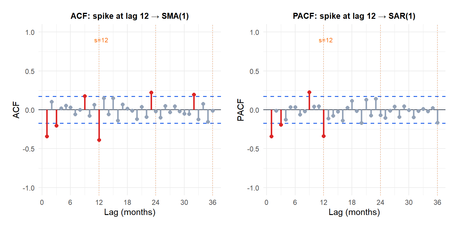
The orange dotted lines mark the seasonal lags (12, 24, 36). The significant spike at lag 12 in the ACF (but not at 24) suggests SMA(1). The spike at lag 12 in the PACF suggests SAR(1). Combined with the non-seasonal structure, this points to SARIMA(0,1,1)(0,1,1)\(_{12}\) or SARIMA(0,1,1)(1,1,0)\(_{12}\).
The airline model: SARIMA(0,1,1)(0,1,1)\(_{12}\)
The most famous SARIMA model, proposed by Box and Jenkins for the airline passenger data:
\[\Delta\Delta_{12}\log y_t = (1 + \theta L)(1 + \Theta L^{12})\varepsilon_t\]
Expanded:
\[\Delta\Delta_{12}\log y_t = \varepsilon_t + \theta\varepsilon_{t-1} + \Theta\varepsilon_{t-12} + \theta\Theta\varepsilon_{t-13}\]
Only two parameters (\(\theta\) and \(\Theta\)) capture both the short-term dynamics and the seasonal pattern. The log transformation stabilizes the growing variance; regular differencing removes the trend; seasonal differencing removes the seasonal trend.
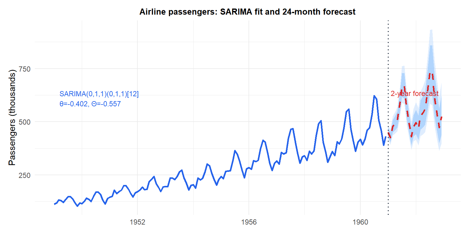
The forecast (red) preserves the seasonal pattern and the upward trend, with prediction intervals that widen appropriately.
Residual diagnostics
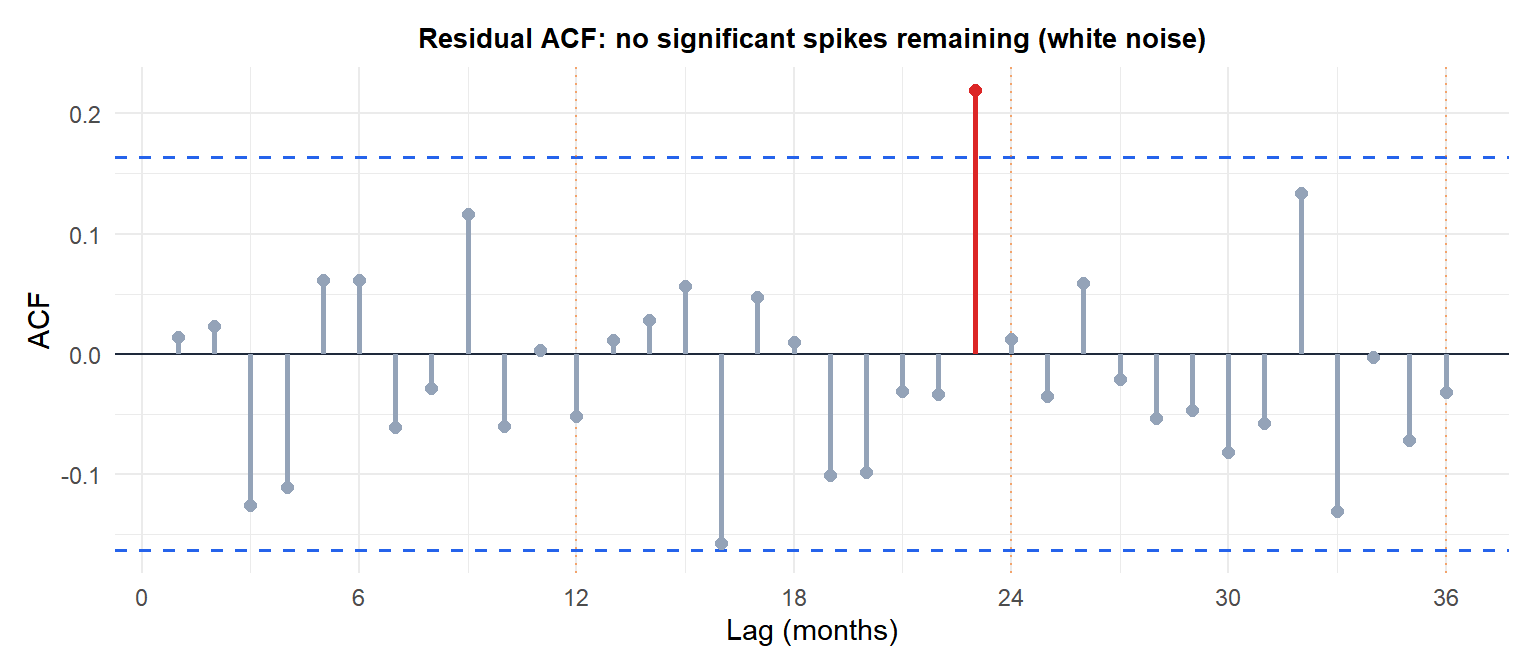
No significant spikes at any lag, including the seasonal lags 12 and 24. The model has captured all the autocorrelation structure.
⚠️ Seasonal over-differencing inflates forecast variance
Applying \(D = 1\) when \(D = 0\) is sufficient introduces a unit root in the seasonal MA, making the model non-invertible and producing forecasts with exploding variance. Signs: the ACF of the seasonally differenced series starts with a large negative value at lag \(s\).
A common mistake for monthly data: applying both \(D = 1\) (seasonal) and \(d = 2\) (non-seasonal) when \(d = 1, D = 1\) suffices. Use forecast::nsdiffs(y) to determine \(D\) and forecast::ndiffs(diff(y, 12)) to determine \(d\) after seasonal differencing.
💡 SARIMA in R
# Fit SARIMA(0,1,1)(0,1,1)[12] manually
arima(log(y), order = c(0,1,1),
      seasonal = list(order = c(0,1,1), period = 12))

# Automatic SARIMA selection
library(forecast)
auto.arima(y, seasonal = TRUE)   # default, searches seasonal orders too

# Determine differencing orders
nsdiffs(y)             # number of seasonal differences needed
ndiffs(diff(y, 12))   # non-seasonal differences after seasonal differencing

# Forecast and plot
fc <- forecast(fit, h = 24)
autoplot(fc)
