Kalman filter
The Kalman filter is a recursive algorithm that estimates the hidden state of a dynamic system from noisy observations. It is optimal under Gaussian assumptions: no other linear estimator has lower mean squared error. Originally developed for aerospace navigation, it is now central to econometrics, signal processing, robotics, and time series analysis.
The state space model
The Kalman filter operates on systems described by two equations:
\[\alpha_{t+1} = T_t \alpha_t + R_t \eta_t \qquad \text{(transition equation)}\]
\[y_t = Z_t \alpha_t + \varepsilon_t \qquad \text{(observation equation)}\]
where:
- \(\alpha_t\): the state vector (unobserved). Contains the quantities we want to estimate: position, level, trend, seasonal components.
- \(y_t\): the observation (noisy measurement of \(\alpha_t\)).
- \(T_t\): transition matrix governing how the state evolves over time.
- \(Z_t\): observation matrix linking the state to the observation.
- \(\eta_t \sim N(0, Q_t)\): state noise (process noise).
- \(\varepsilon_t \sim N(0, H_t)\): observation noise (measurement noise).
- \(\eta_t\) and \(\varepsilon_t\) are mutually independent.
The ratio \(Q/H\) controls the trade-off between trusting the model dynamics (\(Q\) large) and trusting the observations (\(H\) large).
The predict-update algorithm
The Kalman filter runs recursively at each time step \(t\):
Predict (propagate state forward using the transition equation):
\[\hat{\alpha}_{t|t-1} = T_t \hat{\alpha}_{t-1|t-1}\]
\[P_{t|t-1} = T_t P_{t-1|t-1} T_t' + R_t Q_t R_t'\]
Update (incorporate the new observation \(y_t\)):
\[v_t = y_t - Z_t \hat{\alpha}_{t|t-1} \qquad \text{(innovation)}\]
\[F_t = Z_t P_{t|t-1} Z_t' + H_t \qquad \text{(innovation variance)}\]
\[K_t = P_{t|t-1} Z_t' F_t^{-1} \qquad \text{(Kalman gain)}\]
\[\hat{\alpha}_{t|t} = \hat{\alpha}_{t|t-1} + K_t v_t\]
\[P_{t|t} = (I - K_t Z_t) P_{t|t-1}\]
The Kalman gain \(K_t\) controls how much weight to give the new observation vs the prediction:
- \(K_t \to 0\) (small \(H_t\), large \(Q_t\)): trust the model; ignore new observation.
- \(K_t \to 1\) (large \(H_t\), small \(Q_t\)): trust the observation; heavily update state.
The innovation \(v_t = y_t - Z_t\hat{\alpha}_{t|t-1}\) is the one-step prediction error. Under the correct model, innovations are white noise with variance \(F_t\).
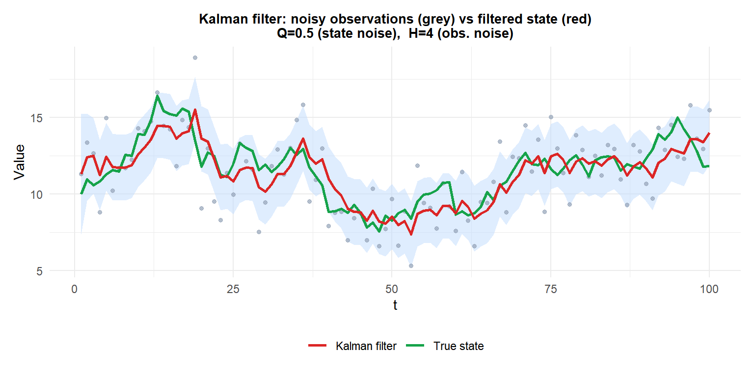
Grey dots: noisy observations. Green: true underlying state (random walk). Red: Kalman filter estimate with 95% uncertainty band. The filter tracks the true state closely despite heavy observation noise.
The Q/H trade-off
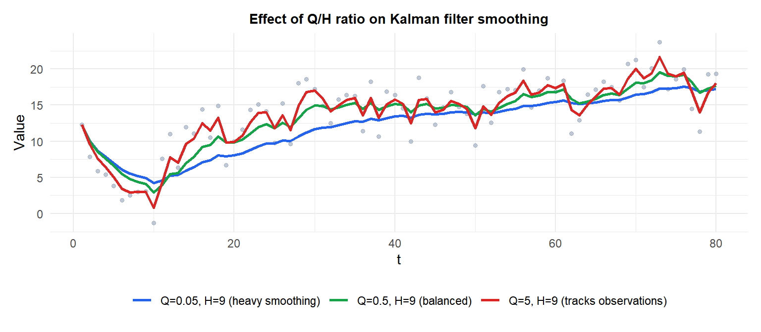
Low Q/H (blue) produces heavy smoothing: the filter is slow to react to changes. High Q/H (red) tracks observations closely. Optimal Q and H are estimated from data by maximum likelihood.
Connection with ARIMA
Every ARIMA model has an exact state space representation. For example, ARIMA(1,1,1):
\[\alpha_t = \begin{pmatrix}\mu_t \\ b_t\end{pmatrix}, \quad T = \begin{pmatrix}1 & 1 \\ 0 & 1\end{pmatrix}, \quad Z = \begin{pmatrix}1 & 0\end{pmatrix}\]
This allows fitting ARIMA models using the Kalman filter, which handles:
- Missing data: the update step is simply skipped when \(y_t\) is missing.
- Exact likelihood computation: the innovations \(v_t\) and their variances \(F_t\) give the Gaussian log-likelihood directly: \(\ell = -\frac{1}{2}\sum_t (\log F_t + v_t^2/F_t)\).
- Non-stationary initialization: diffuse priors handle \(I(1)\) or \(I(2)\) components without pre-differencing.
The stats::arima() and forecast::Arima() functions in R use the Kalman filter internally.
Filtering, smoothing and forecasting
The Kalman filter produces three types of state estimates:
- Filtered estimate \(\hat{\alpha}_{t|t}\): uses all data up to \(t\). Real-time estimate.
- Smoothed estimate \(\hat{\alpha}_{t|T}\): uses all data up to \(T > t\). Retrospective; always more precise than filtered.
- Forecast \(\hat{\alpha}_{t+h|t}\): projects forward from \(t\) using only the transition equation.
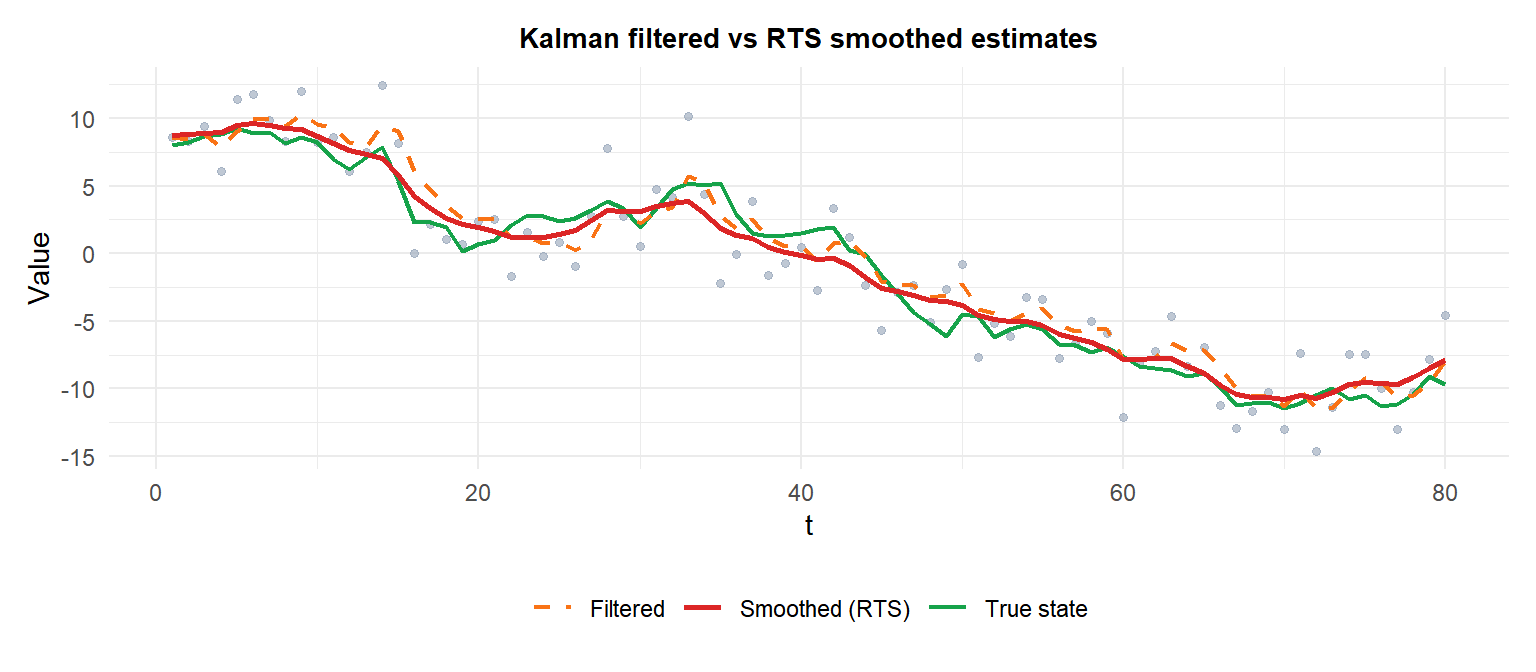
The smoothed estimate (red) is always closer to the true state than the filtered estimate (orange) because it uses all \(T\) observations, not just those up to \(t\).
⚠️ Misspecified Q and H lead to poor filtering
The Kalman filter is optimal only when \(Q\) and \(H\) are correctly specified. Common problems:
- Q too small: the filter is overconfident in its predictions and slow to track real changes in the state.
- H too small: the filter trusts observations too much, producing noisy estimates that follow every measurement fluctuation.
- Both misspecified: the innovation sequence \(v_t\) will not be white noise. Always check the ACF of innovations after fitting.
Estimate \(Q\) and \(H\) by maximum likelihood (maximize \(\ell = -\frac{1}{2}\sum_t (\log F_t + v_t^2/F_t)\)) using numerical optimization. In R, dlm::dlmMLE() or KFAS::fitSSM() do this automatically.
💡 Kalman filter in R
# Via ARIMA (Kalman filter used internally)
arima(y, order = c(1,1,1))

# Explicit state space with dlm package
library(dlm)
model <- dlmModPoly(order = 1, dV = H, dW = Q)  # local level model
filtered  <- dlmFilter(y, model)
smoothed  <- dlmSmooth(filtered)

# KFAS package (more flexible)
library(KFAS)
model <- SSModel(y ~ SSMtrend(1, Q = Q), H = H)
out   <- KFS(model)   # filtering + smoothing in one call
