Holt-Winters method
The Holt-Winters method extends exponential smoothing to series with both trend and seasonality by maintaining three smoothed components: level \(\ell_t\), trend \(b_t\), and seasonal index \(s_t\). It comes in additive and multiplicative variants depending on how seasonality interacts with the level.
Additive Holt-Winters
Use when seasonal fluctuations are roughly constant in absolute terms regardless of the level of the series.
\[\ell_t = \alpha(y_t - s_{t-m}) + (1-\alpha)(\ell_{t-1} + b_{t-1})\]
\[b_t = \beta(\ell_t - \ell_{t-1}) + (1-\beta)b_{t-1}\]
\[s_t = \gamma(y_t - \ell_{t-1} - b_{t-1}) + (1-\gamma)s_{t-m}\]
\[\hat{y}_{t+h} = \ell_t + h \cdot b_t + s_{t+h-m}\]
where \(m\) is the season length and \(\alpha, \beta, \gamma \in (0,1)\) are the smoothing parameters for level, trend and seasonality respectively. The seasonal index \(s_t\) is updated using the deviation of \(y_t\) from the detrended level.
Multiplicative Holt-Winters
Use when seasonal fluctuations grow proportionally with the level (e.g., airline passengers, retail sales that scale with volume).
\[\ell_t = \alpha\frac{y_t}{s_{t-m}} + (1-\alpha)(\ell_{t-1} + b_{t-1})\]
\[b_t = \beta(\ell_t - \ell_{t-1}) + (1-\beta)b_{t-1}\]
\[s_t = \gamma\frac{y_t}{\ell_{t-1} + b_{t-1}} + (1-\gamma)s_{t-m}\]
\[\hat{y}_{t+h} = (\ell_t + h \cdot b_t) \cdot s_{t+h-m}\]
The multiplicative model divides by the seasonal index instead of subtracting it. Seasonal indices fluctuate around 1 (values above 1 indicate above-average periods; below 1 indicate below-average). The additive model’s indices fluctuate around 0.
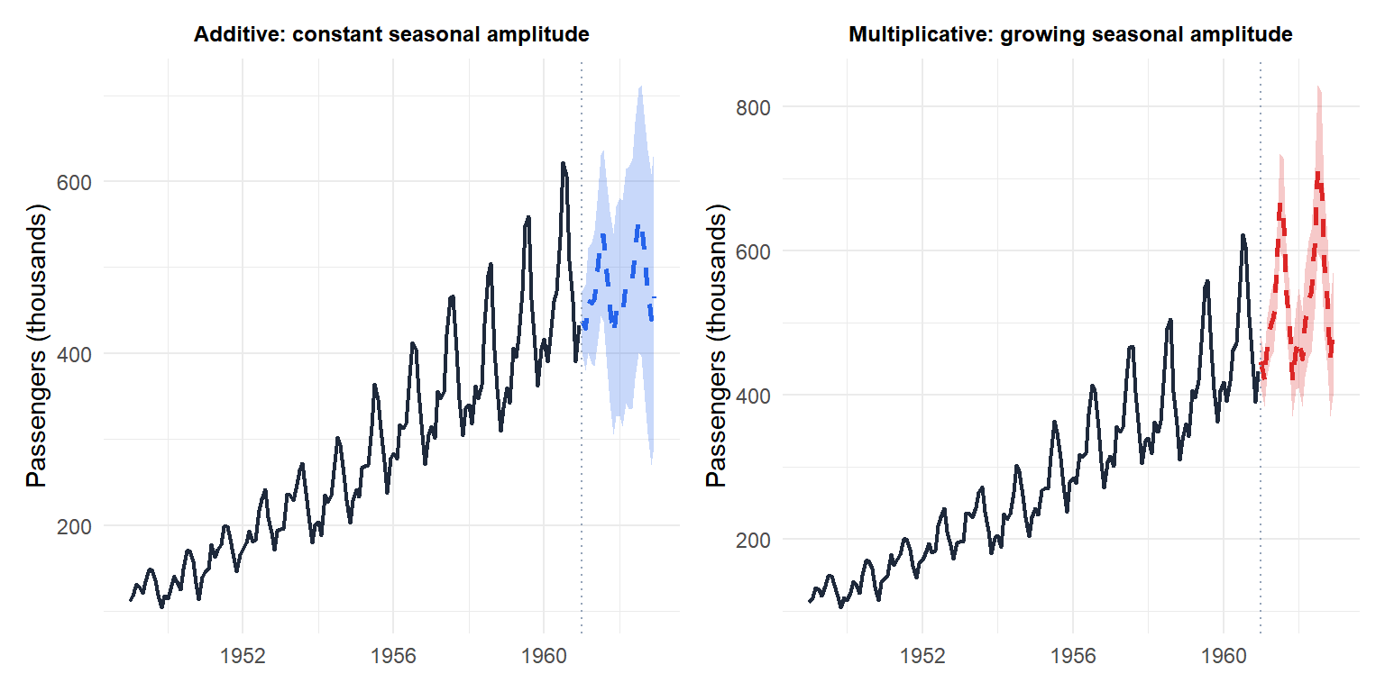
The additive model (left) forecasts seasonal swings of constant size. The multiplicative model (right) forecasts swings that grow with the level, which matches the historical pattern better for airline data.
Initialization
Proper initialization is essential: poor starting values can take many periods to correct. The standard approach:
Level \(\ell_m\): average of the first complete season: \[\ell_m = \frac{1}{m}\sum_{i=1}^m y_i\]
Trend \(b_m\): average of the first-season-to-second-season changes: \[b_m = \frac{1}{m}\left(\frac{y_{m+1}-y_1}{m} + \frac{y_{m+2}-y_2}{m} + \cdots + \frac{y_{2m}-y_m}{m}\right)\]
Seasonal indices \(s_1, \ldots, s_m\) (additive): deviation of each period from the first-season average: \[s_i = y_i - \ell_m, \quad i = 1, \ldots, m\]
For multiplicative: \(s_i = y_i / \ell_m\).
In practice, R’s HoltWinters() and ets() estimate initial values jointly with the smoothing parameters by minimizing SSE.
Damped trend Holt-Winters
Holt-Winters with a linear trend can over-forecast at long horizons: the trend is extrapolated indefinitely. The damped trend variant introduces a damping parameter \(\phi \in (0,1)\) that flattens the trend over time:
\[\hat{y}_{t+h} = \ell_t + (\phi + \phi^2 + \cdots + \phi^h)b_t + s_{t+h-m}\]
As \(h \to \infty\), the bracketed sum converges to \(\phi/(1-\phi)\), so the forecast asymptotes to a constant level. Damped trend typically gives better performance at medium and long horizons than undamped Holt-Winters.
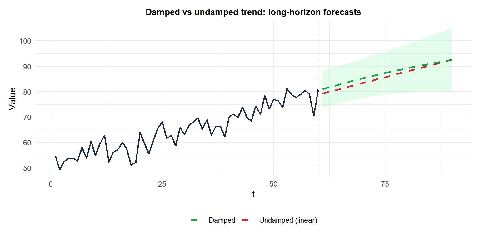
The undamped forecast (red) extrapolates the trend linearly without limit. The damped forecast (green) flattens toward a constant level, which is usually more realistic at horizons beyond 1-2 seasons.
Choosing additive vs multiplicative
| Criterion | Additive | Multiplicative |
|---|---|---|
| Seasonal amplitude | Constant over time | Grows with level |
| Log-transformed data | Either works | Additive on log \(\equiv\) multiplicative on original |
| Negative values possible | Yes | No (\(y_t > 0\) required) |
| ETS notation | ETS(A,A,A) | ETS(M,A,M) or ETS(A,A,M) |
A practical rule: plot the series and check whether the seasonal swings widen as the series grows. If yes, use multiplicative (or log-transform and use additive).
⚠️ Multiplicative model requires strictly positive data
The multiplicative Holt-Winters divides by \(s_{t-m}\) and \(\ell_{t-1} + b_{t-1}\), which requires all values to be strictly positive. If the series contains zeros or negative values (counts with zeros, temperature in Celsius), use the additive model or transform the data.
Also, the multiplicative model can become unstable if the level approaches zero during the recursion, producing explosive seasonal indices.
Fitting Holt-Winters in R
# Base R
fit_add  <- HoltWinters(y, seasonal = "additive")
fit_mult <- HoltWinters(y, seasonal = "multiplicative")

# forecast package (recommended: automatic parameter optimization)
library(forecast)
fit <- hw(y, h = 24, seasonal = "multiplicative", damped = TRUE)
forecast(fit, h = 24)

# ETS framework (automatic model selection)
fit_ets <- ets(y)          # selects best ETS model by AIC
summary(fit_ets)           # shows selected model, e.g. ETS(M,Ad,M)
forecast(fit_ets, h = 24)
💡 Let AIC choose between additive and multiplicative
Rather than choosing manually, fit both models and compare AIC:
fit_a <- ets(y, model = "AAA")   # additive
fit_m <- ets(y, model = "MAM")   # multiplicative (mult. error + seas.)
AIC(fit_a); AIC(fit_m)
Or use ets(y) which searches automatically. The selected model is shown as ETS(error, trend, season), e.g. ETS(M,Ad,M) means multiplicative error, additive damped trend, multiplicative seasonality.

