Autoregressive moving average model (ARMA)
The ARMA(\(p,q\)) model combines \(p\) autoregressive terms and \(q\) moving average terms into a single framework. It is more parsimonious than using a pure AR or MA model alone: many processes that require a high-order AR or MA can be represented exactly or approximately by a low-order ARMA. It applies to stationary series only.
Definition
\[y_t = \phi_1 y_{t-1} + \cdots + \phi_p y_{t-p} + \varepsilon_t + \theta_1 \varepsilon_{t-1} + \cdots + \theta_q \varepsilon_{t-q}\]
In lag operator notation:
\[\Phi(L)\,y_t = \Theta(L)\,\varepsilon_t\]
\[\Phi(L) = 1 - \phi_1 L - \cdots - \phi_p L^p, \qquad \Theta(L) = 1 + \theta_1 L + \cdots + \theta_q L^q\]
The AR polynomial \(\Phi(L)\) acts on \(y_t\); the MA polynomial \(\Theta(L)\) acts on \(\varepsilon_t\).
Stationarity and invertibility
An ARMA(\(p,q\)) is:
- Stationary if all roots of \(\Phi(z) = 0\) lie outside the unit circle (same condition as pure AR(\(p\))).
- Invertible if all roots of \(\Theta(z) = 0\) lie outside the unit circle (same condition as pure MA(\(q\))).
- Identifiable: there must be no common roots between \(\Phi(z)\) and \(\Theta(z)\) (no cancellation). If a root is shared, the effective order is lower and the model is overparameterized.
⚠️ Common factor cancellation: the parameter redundancy trap
If \(\Phi(z)\) and \(\Theta(z)\) share a common root, the true model is of lower order. For example, ARMA(2,1) with \(\phi_1 = 0.9\), \(\phi_2 = -0.2\), \(\theta_1 = 0.4\): if \(z = 0.5\) is a root of both polynomials, the model actually reduces to ARMA(1,0). Fitting the overparameterized model produces large standard errors and instability.
Symptom: if fitted \(\phi\) and \(\theta\) coefficients are close in magnitude with opposite signs on the same lag, suspect cancellation. Check by computing the roots of both polynomials.
Why ARMA is more parsimonious
By Wold’s decomposition theorem, any stationary process can be represented as MA(\(\infty\)). An ARMA(\(p,q\)) provides a rational approximation using only \(p+q\) parameters instead of infinitely many.
A classic example: the MA(\(\infty\)) representation of AR(1) is:
\[y_t = \varepsilon_t + \phi\varepsilon_{t-1} + \phi^2\varepsilon_{t-2} + \cdots\]
which requires infinitely many MA parameters. The ARMA(1,0) captures this with just one parameter \(\phi\).
Conversely, some processes that look like high-order AR or MA in the ACF/PACF can be represented exactly by a low-order ARMA. This is the principal motivation for using ARMA over pure AR or MA.
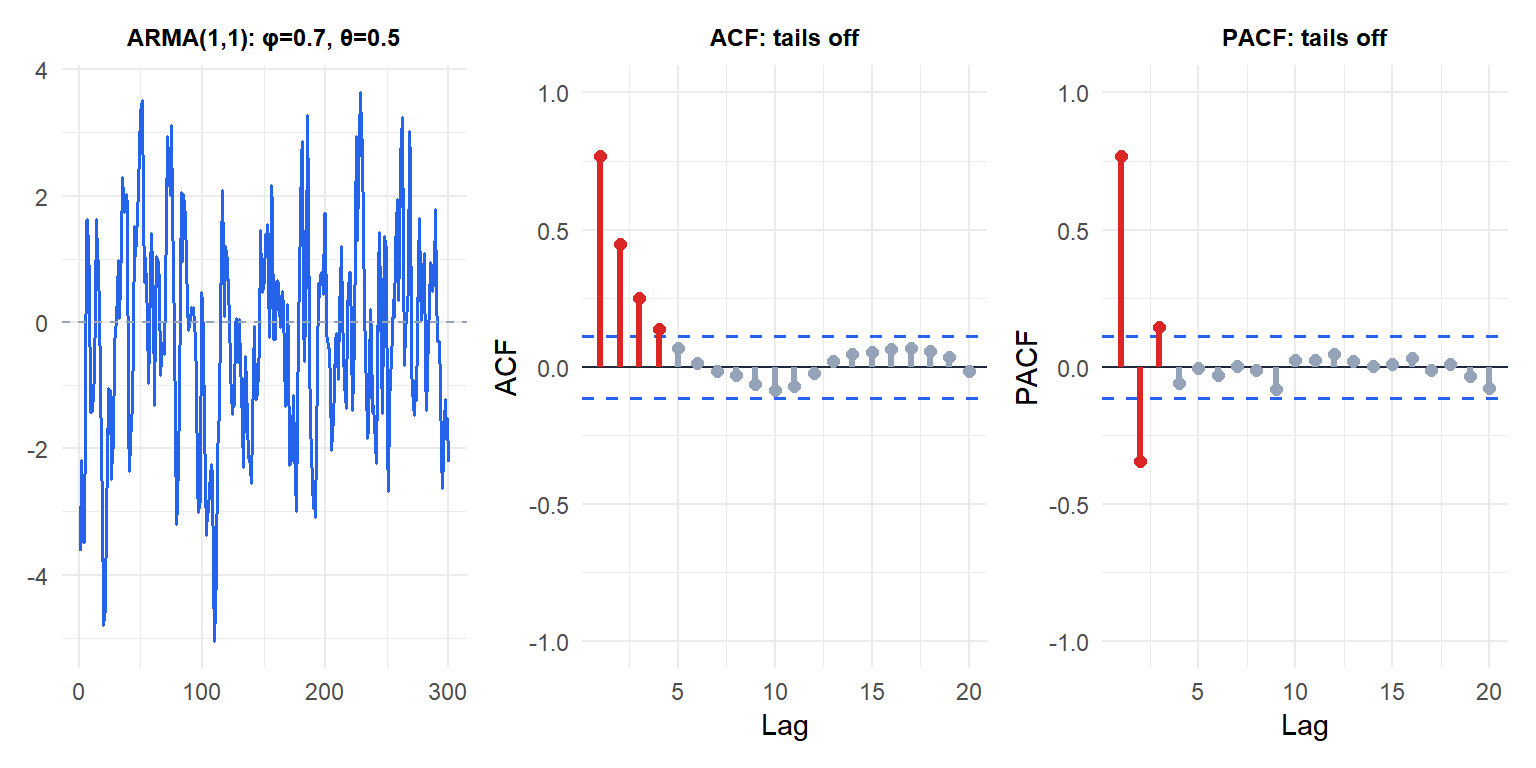
Both ACF and PACF tail off gradually, confirming the ARMA structure. Neither cuts off sharply, which is why pure AR or MA identification would require high orders.
Order selection: AIC and BIC
For ARMA(\(p,q\)), ACF/PACF identification is less clear-cut than for pure AR or MA. The standard approach is to fit several candidate models and compare by:
\[\text{AIC} = -2\log\hat{L} + 2(p+q+1), \qquad \text{BIC} = -2\log\hat{L} + \log(T)(p+q+1)\]
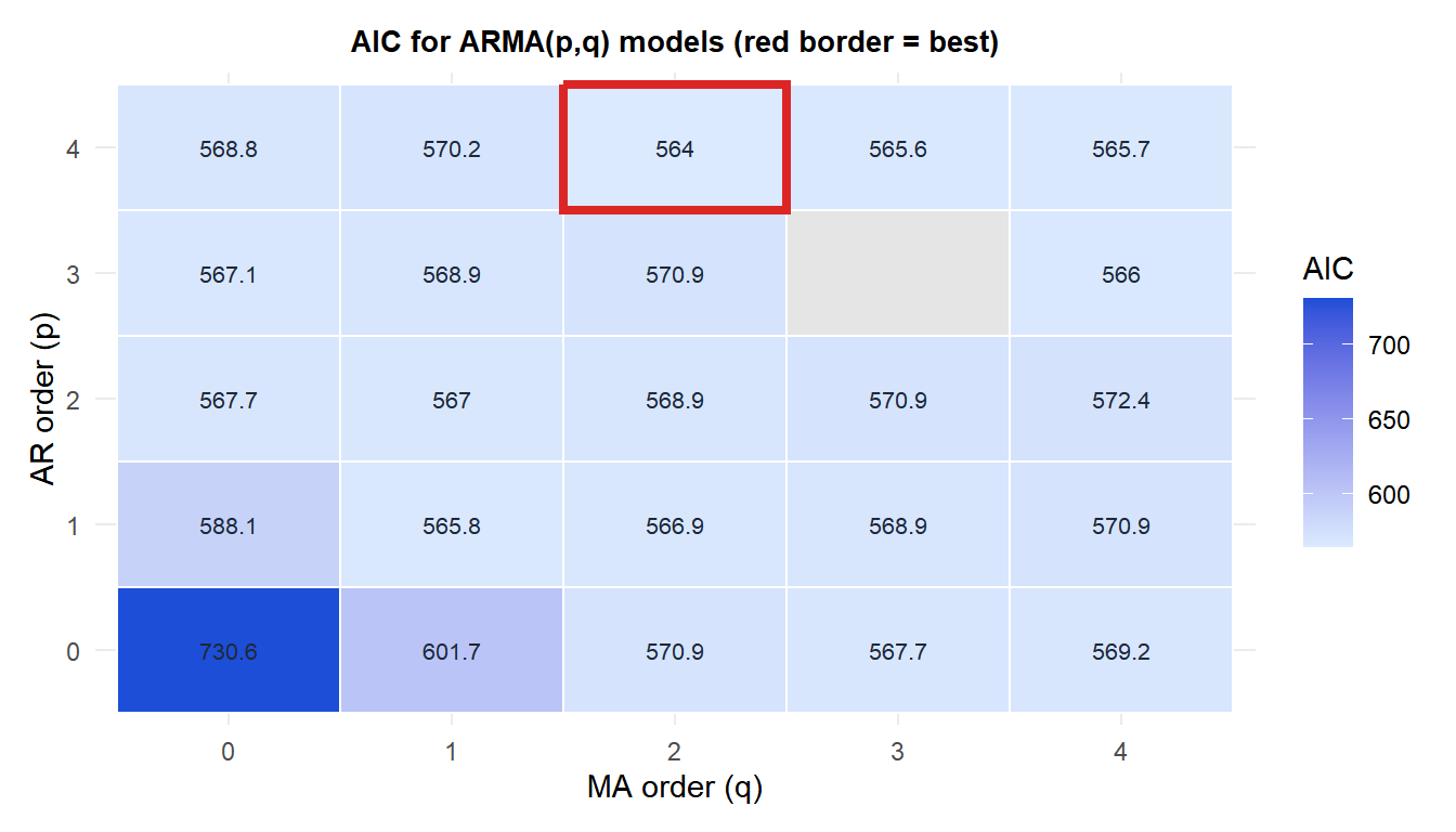
The heatmap shows AIC across a grid of AR and MA orders. Lower AIC (darker blue) indicates better fit penalized for complexity. The red border marks the best model. High-order models in the top-right corner show worse AIC despite more parameters.
Example: ARMA(1,1) for monthly sales
Monthly sales data often exhibit both persistence (AR component) and correction after forecast errors (MA component). An ARMA(1,1) captures both with just two parameters.
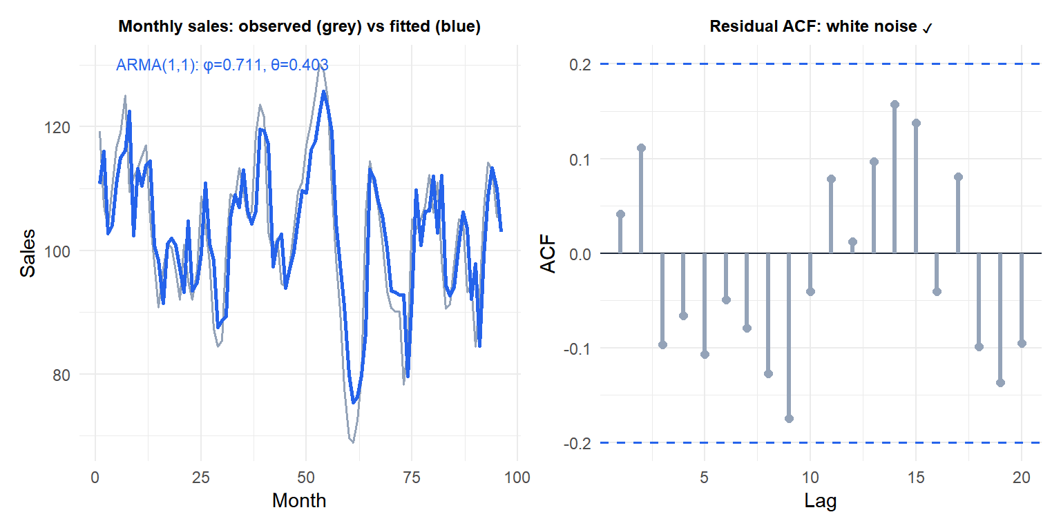
The residual ACF shows no significant spikes: the ARMA(1,1) has captured the autocorrelation structure. Confirm with the Ljung-Box test: Box.test(residuals(fit), lag = 20, type = "Ljung-Box", fitdf = 2).
💡 Fitting ARMA models in R
# Fit ARMA(1,1)
fit <- arima(y, order = c(1, 0, 1))
summary(fit)

# Automatic selection by AIC
library(forecast)
auto.arima(y, d = 0, max.p = 4, max.q = 4, stationary = TRUE)

# Check residuals
checkresiduals(fit)   # plots residuals, ACF and Ljung-Box p-value

