ARIMAX model
ARIMAX adds external (exogenous) regressors to the ARIMA framework. It is the natural model when the time series is driven not only by its own past values but also by observable external factors such as price, temperature, or promotional spend.
Why exogenous variables?
Pure ARIMA models exploit only the autocorrelation structure of the series. Many real series are also driven by external factors:
- Electricity demand depends on temperature.
- Retail sales depend on price promotions and holidays.
- Website traffic depends on advertising spend.
- Airline bookings depend on fuel prices and economic indicators.
Including these variables as regressors can dramatically improve forecast accuracy when their future values are known or can be predicted independently.
Two related but different models
There are two models commonly called ARIMAX, and they are mathematically distinct:
Model 1: ARIMAX (true exogenous model)
The exogenous variables \(x_t\) enter the differenced equation directly:
\[\Phi(L)(1-L)^d y_t = \beta x_t + \Theta(L)\varepsilon_t\]
The AR and MA polynomials operate on the differenced \(y_t\). The regressor \(x_t\) is not differenced. This is a restricted model: it assumes \(x_t\) is strictly exogenous and does not feed back into \(y_t\).
Model 2: Regression with ARIMA errors (recommended)
The regression happens first, and the ARIMA model is applied to the residuals:
\[y_t = \beta x_t + \eta_t, \qquad \Phi(L)(1-L)^d\eta_t = \Theta(L)\varepsilon_t\]
Here \(\eta_t\) follows an ARIMA process. The regressor enters the undifferenced series, and differencing applies only to the error process. This is the formulation used by forecast::auto.arima() with xreg.
⚠️ ARIMAX and regression with ARIMA errors are not the same model
The key difference: in Model 1 the differencing operator applies to \(\beta x_t y_t\), meaning \(x_t\) is also implicitly differenced. In Model 2, \(x_t\) enters the level equation and only the errors are differenced.
In practice, Model 2 (regression with ARIMA errors) is almost always preferred because:
- The coefficient \(\beta\) has a direct interpretation as the effect of \(x_t\) on \(y_t\) in levels.
- It handles non-stationary \(y_t\) without requiring \(x_t\) to be differenced.
- It is what
Arima(y, xreg = x)andauto.arima(y, xreg = x)actually fit in R.
When people say ARIMAX in applied work, they usually mean Model 2.
Example: electricity demand and temperature
Half-hourly electricity demand is strongly driven by temperature (heating and cooling effects). We model daily peak demand as a function of daily mean temperature, with ARIMA errors capturing the remaining autocorrelation.
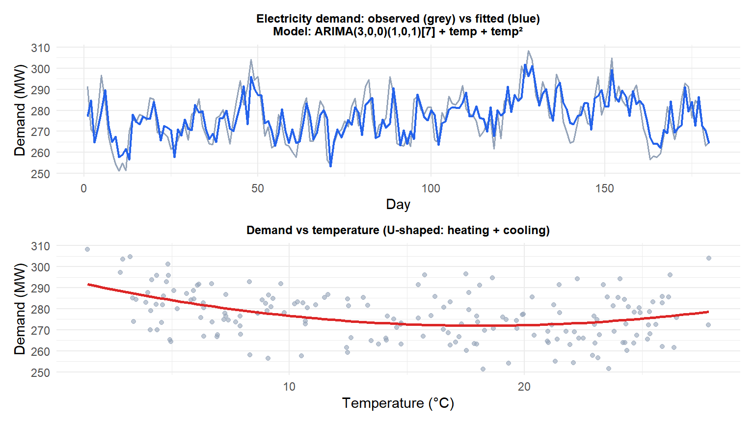
The U-shaped relationship (cooling demand at high temperatures, heating demand at low temperatures) is captured by including both \(\text{temp}\) and \(\text{temp}^2\) as regressors. The ARIMA component handles the remaining weekly autocorrelation.
Forecasting with ARIMAX
To forecast \(h\) steps ahead, future values of the exogenous variables must be provided:
# Future temperature scenarios
temp_future <- c(22, 24, 25, 26, 28, 27, 23)  # next 7 days
xreg_future <- cbind(temp = temp_future,
                     temp2 = temp_future^2)

forecast(fit_x, xreg = xreg_future, h = 7)
This is the key practical constraint of ARIMAX: the forecast is conditional on the future regressor values. If the regressor is itself uncertain (e.g., temperature forecast), the uncertainty in \(x_t\) must be propagated into the forecast intervals.
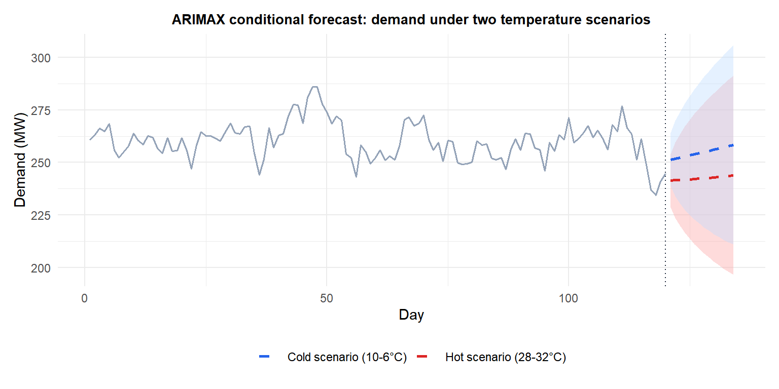
The two scenarios produce very different demand forecasts, illustrating the value of incorporating temperature as a regressor. ARIMA alone would produce a single forecast without this conditional structure.
When to use ARIMAX
| Situation | Recommended model |
|---|---|
| \(y_t\) depends on known external \(x_t\) | ARIMAX (regression with ARIMA errors) |
| \(y_t\) and \(x_t\) mutually influence each other | VAR (vector autoregression) |
| Only autocorrelation, no externals | ARIMA |
| Seasonal + external factors | SARIMAX (seasonal ARIMAX) |
| Non-linear relationship with \(x_t\) | Include \(x_t^2\), interactions, or use ML models |
💡 ARIMAX in R
library(forecast)

# Fit regression with ARIMA errors
fit <- auto.arima(y, xreg = x_matrix)

# Manual specification
Arima(y, order = c(1,1,1), xreg = x_matrix)

# Forecast (must supply future xreg values)
forecast(fit, xreg = x_future, h = nrow(x_future))

# Check residuals as usual
checkresiduals(fit)
The xreg argument accepts a matrix of regressors. Each column is one regressor. R fits Model 2 (regression with ARIMA errors), not the pure ARIMAX formulation.

