ARIMA model
ARIMA(\(p,d,q\)) extends ARMA(\(p,q\)) to non-stationary series by differencing \(d\) times. The \(d\) differences remove stochastic trends (unit roots), leaving a stationary series to which the ARMA(\(p,q\)) is applied. It is the most widely used model class for univariate time series forecasting.
Definition
A series \(y_t\) follows an ARIMA(\(p,d,q\)) if \(w_t = \Delta^d y_t = (1-L)^d y_t\) follows a stationary ARMA(\(p,q\)):
\[\Phi(L)(1-L)^d y_t = \Theta(L)\varepsilon_t\]
\[\Phi(L) = 1 - \phi_1 L - \cdots - \phi_p L^p, \qquad \Theta(L) = 1 + \theta_1 L + \cdots + \theta_q L^q\]
The three parameters:
- \(p\): AR order (number of autoregressive lags).
- \(d\): degree of differencing (integration order). \(d=0\) gives ARMA; \(d=1\) is the most common case.
- \(q\): MA order (number of moving average terms).
Special cases: ARIMA(1,0,0) = AR(1); ARIMA(0,1,0) = random walk; ARIMA(0,1,1) = exponentially weighted moving average (EWMA).
The Box-Jenkins methodology
The systematic procedure for identifying and fitting ARIMA models, proposed by Box and Jenkins (1970):
Step 1: Identification. Plot the series. Apply log or Box-Cox if variance is non-constant. Test for unit roots (ADF, KPSS). Difference \(d\) times until stationary. Examine ACF and PACF of the differenced series to identify candidate \(p\) and \(q\).
Step 2: Estimation. Fit the candidate ARIMA(\(p,d,q\)) by MLE. Compare models by AIC and BIC.
Step 3: Diagnostics. Check residuals are white noise: ACF of residuals, Ljung-Box test. If residuals show autocorrelation, revise \(p\) or \(q\).
Step 4: Forecasting. Use the fitted model to produce point forecasts and prediction intervals.
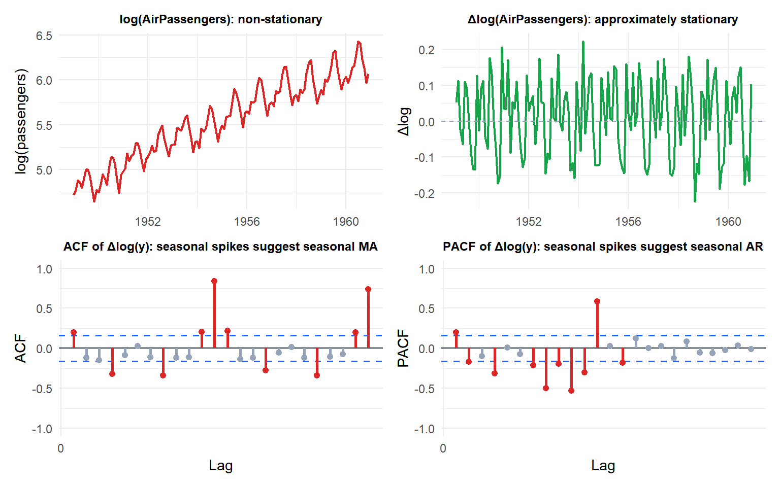
The original log series is non-stationary (upward trend). After one difference it is approximately stationary. The ACF and PACF of \(\Delta\log(y)\) still show seasonal spikes at lags 12, 24, suggesting a seasonal extension (SARIMA) is needed.
Choosing d
\(d\) is determined by unit root testing:
- Apply ADF and KPSS to the original series.
- If non-stationary, difference once and retest.
- Stop when both tests agree the series is stationary.
- For most economic and financial series, \(d = 1\) suffices. \(d = 2\) is rare and often indicates over-differencing.
In R: forecast::ndiffs(y) automates this using sequential ADF tests.
⚠️ Over-differencing makes forecasts worse
Applying \(d = 2\) when \(d = 1\) is sufficient introduces a unit root in the MA polynomial, producing unstable parameter estimates and forecasts that fan out excessively. Signs of over-differencing: the ACF of \(\Delta^d y_t\) starts at a large negative value at lag 1.
Under-differencing (using \(d = 0\) for a series that needs \(d = 1\)) produces non-stationary residuals with drifting mean and growing variance.
Example: ARIMA(1,1,1)
Fit an ARIMA(1,1,1) to the monthly US unemployment rate (a classic non-stationary economic series).
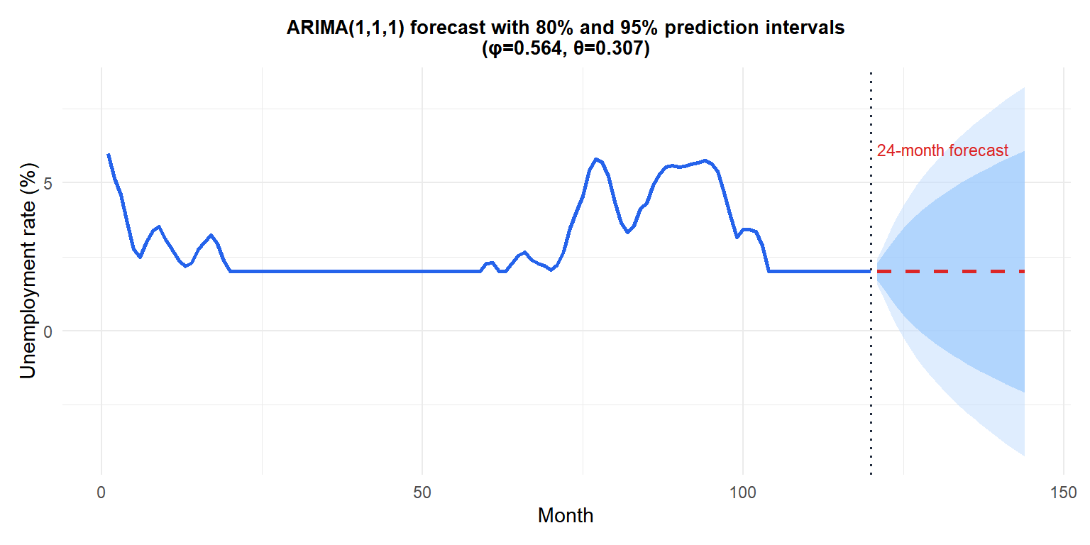
Prediction intervals widen with horizon: ARIMA(1,1,1) forecasts revert toward the recent trend, with uncertainty growing linearly in variance. The 80% (darker) and 95% (lighter) bands reflect this.
ARIMA vs ARMA
| ARMA(\(p,q\)) | ARIMA(\(p,d,q\)) | |
|---|---|---|
| Requires stationarity | Yes | No (handles \(I(d)\) series) |
| Handles trends | No | Yes (via differencing) |
| Long-run forecast | Reverts to constant mean | Follows a stochastic trend |
| \(d = 0\) special case | Yes (ARIMA = ARMA) | - |
💡 ARIMA in R
# Manual specification
arima(y, order = c(1, 1, 1))

# Automatic selection by AIC (Box-Jenkins automated)
library(forecast)
auto.arima(y)

# Diagnose residuals
checkresiduals(fit)

# Forecast 12 periods ahead
forecast(fit, h = 12)
auto.arima() applies the Box-Jenkins methodology automatically: it tests for unit roots to choose \(d\), then searches over \((p, q)\) by AIC. It is the recommended starting point for any ARIMA analysis.

