ACF and PACF
The ACF measures the correlation between \(y_t\) and \(y_{t-k}\) at each lag \(k\). The PACF measures the same correlation after removing the effect of all intermediate lags. Together they are the primary diagnostic tools for identifying AR and MA orders before fitting a model.
Autocorrelation function (ACF)
The autocorrelation at lag \(k\) is the correlation between \(y_t\) and \(y_{t-k}\):
\[\rho_k = \frac{\text{Cov}(y_t, y_{t-k})}{\text{Var}(y_t)} = \frac{\gamma_k}{\gamma_0}\]
where \(\gamma_k = \text{Cov}(y_t, y_{t-k})\) is the autocovariance at lag \(k\) and \(\gamma_0 = \text{Var}(y_t)\). By definition, \(\rho_0 = 1\).
The sample ACF estimates \(\rho_k\) from data:
\[\hat{\rho}_k = \frac{\sum_{t=k+1}^T (y_t - \bar{y})(y_{t-k} - \bar{y})}{\sum_{t=1}^T (y_t - \bar{y})^2}\]
Under the null hypothesis of no autocorrelation, \(\hat{\rho}_k \approx N(0, 1/T)\) for large \(T\). The 95% confidence bands in ACF plots are \(\pm 1.96/\sqrt{T}\): spikes beyond these bands indicate significant autocorrelation.
Partial autocorrelation function (PACF)
The partial autocorrelation at lag \(k\) is the correlation between \(y_t\) and \(y_{t-k}\) after removing the linear effects of \(y_{t-1}, y_{t-2}, \ldots, y_{t-k+1}\):
\[\phi_{kk} = \text{Corr}(y_t - \hat{y}_t,\; y_{t-k} - \hat{y}_{t-k})\]
where \(\hat{y}_t\) is the projection of \(y_t\) on \(\{y_{t-1}, \ldots, y_{t-k+1}\}\). It answers: “is there a direct relationship between \(y_t\) and \(y_{t-k}\), beyond what is explained by the intermediate values?”
The PACF is estimated by fitting successive AR models and recording the last coefficient:
\[\phi_{kk} = \text{coefficient on } y_{t-k} \text{ in AR}(k) \text{ fit}\]
ACF and PACF patterns for model identification
The theoretical ACF and PACF of AR and MA processes have characteristic patterns that guide model selection:
| Process | ACF | PACF |
|---|---|---|
| AR(\(p\)) | Decays geometrically (tails off) | Cuts off after lag \(p\) |
| MA(\(q\)) | Cuts off after lag \(q\) | Decays geometrically (tails off) |
| ARMA(\(p,q\)) | Tails off after lag \(q-p\) | Tails off after lag \(p-q\) |
| White noise | No significant spikes | No significant spikes |
| Random walk | Slow decay, all large | First spike significant only |
“Cuts off” means the function drops to near zero abruptly after a certain lag. “Tails off” means it decays gradually (geometrically or sinusoidally).
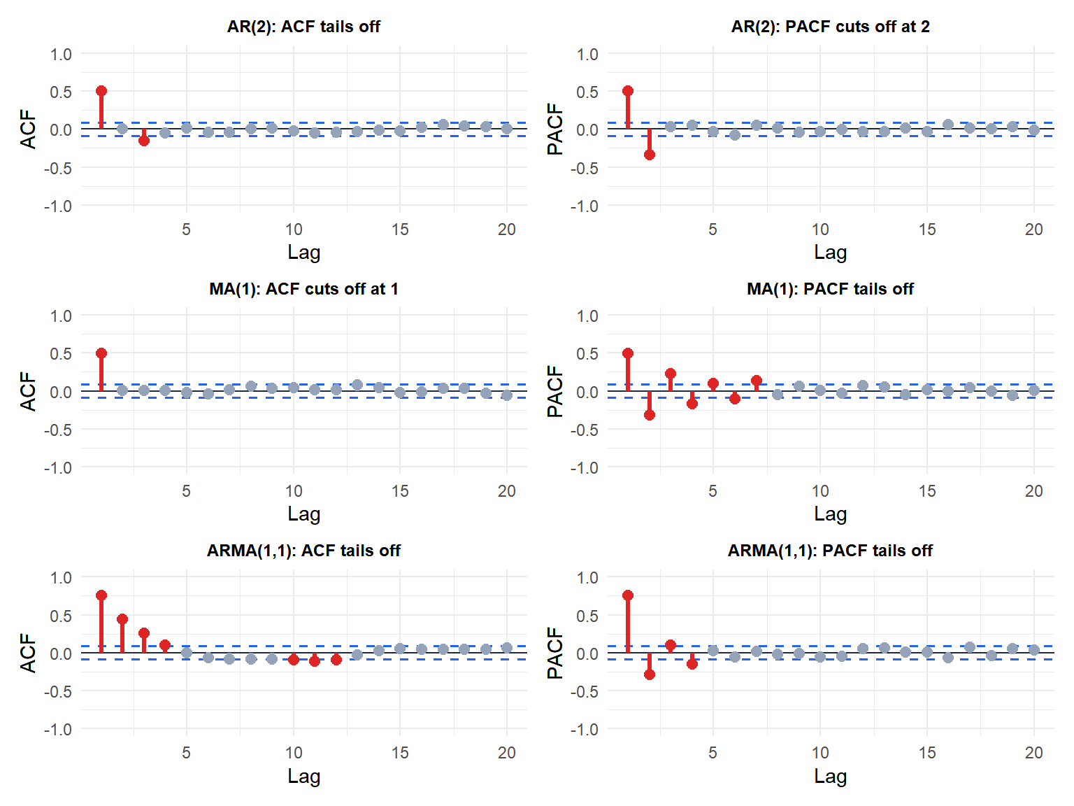
The patterns are clear: AR(2) has PACF cutting off at lag 2; MA(1) has ACF cutting off at lag 1; ARMA(1,1) shows both ACF and PACF tailing off gradually.
Using ACF and PACF to identify model order
The workflow:
- Ensure the series is stationary (difference if needed).
- Plot ACF and PACF.
- Apply the identification rules from the table above.
- Fit candidate models and compare by AIC/BIC.
A series shows:
- ACF: spikes at lags 1, 2, 3 with exponential decay (alternating signs if \(\phi < 0\), same sign if \(\phi > 0\)).
- PACF: single spike at lag 1, nothing significant afterward.
This pattern is consistent with AR(1). Fit arima(y, order = c(1,0,0)) and check residuals.
A series shows:
- ACF: significant spikes at lags 1 and 2, then nothing.
- PACF: gradual decay with alternating pattern.
This pattern is consistent with MA(2). Fit arima(y, order = c(0,0,2)) and check residuals.
Real data example: airline passengers
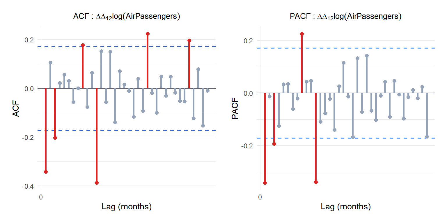
After seasonal and regular differencing, the ACF shows significant spikes at lags 1 and 12 (seasonal), suggesting MA(1) and SMA(1) components. The PACF has spikes at lag 12, consistent with SAR(1). This led to the classic SARIMA(0,1,1)(0,1,1)[12] model for airline data.
⚠️ ACF and PACF patterns are guidelines, not rules
Real data rarely shows perfect textbook patterns. The ACF/PACF suggest candidate models, not definitive answers. Always:
- Fit several candidate models.
- Compare by AIC and BIC.
- Check that residuals are white noise (ACF of residuals, Ljung-Box test).
- Prefer simpler models when AIC/BIC differences are small.
The combination of ACF/PACF inspection with information criteria is more reliable than either alone.
💡 ACF and PACF in R
# Plot ACF and PACF
acf(y, lag.max = 30)
pacf(y, lag.max = 30)

# Numeric values
acf_vals  <- acf(y, lag.max = 30, plot = FALSE)$acf
pacf_vals <- pacf(y, lag.max = 30, plot = FALSE)$acf

# Confidence bands width
ci <- qnorm(0.975) / sqrt(length(y))

# Combined plot with forecast package
library(forecast)
tsdisplay(y)   # shows series + ACF + PACF in one figure
