Unidimensional random variables
A random variable is a function that assigns a numerical value to each outcome of a random experiment. Unidimensional random variables map those outcomes to a single real number, which is the most common case in introductory probability and statistics.
Definition
Informally, a random variable is a way of turning the outcomes of a random experiment into numbers. Roll a die: assign 1 through 6 to each face. Measure a person’s height: record it in centimeters. In both cases, you have a rule that maps each possible outcome to a number.
Formally, given a probability space \((\Omega, \mathcal{A}, P)\), a random variable is a measurable function:
\[X: \Omega \rightarrow \mathbb{R}\]
such that for any Borel set \(B \subseteq \mathbb{R}\):
\[X^{-1}(B) = \{\omega \in \Omega \mid X(\omega) \in B\} \in \mathcal{A}\]
This measurability condition ensures that it makes sense to talk about the probability of \(X\) taking values in any interval or set.
- Rolling a fair die: \(\Omega = \{1,2,3,4,5,6\}\), \(X(\omega) = \omega\). The variable is the result of the roll.
- Flipping a coin 10 times: \(X\) = number of heads. The sample space has \(2^{10}\) outcomes but \(X\) maps them all to \(\{0, 1, \ldots, 10\}\).
- Measuring waiting time at a call center: \(X\) = time in seconds until the call is answered. \(X\) can take any positive real value.
The key distinction between random variables is whether the set of possible values is countable or not.
Discrete random variables
A random variable is discrete when it can only take a finite or countably infinite set of values, typically integers.
Probability mass function (PMF)
The probability mass function assigns a probability to each possible value:
\[ P(X = x_i) = p_i, \quad \text{with } \sum_{i} p_i = 1 \text{ and } p_i \geq 0 \]
Cumulative distribution function (CDF)
The cumulative distribution function gives the probability that \(X\) takes a value less than or equal to \(x\):
\[F(x) = P(X \leq x) = \sum_{x_i \leq x} p_i\]
For discrete variables, the CDF is a step function: it stays flat between consecutive values and jumps at each possible value of \(X\).
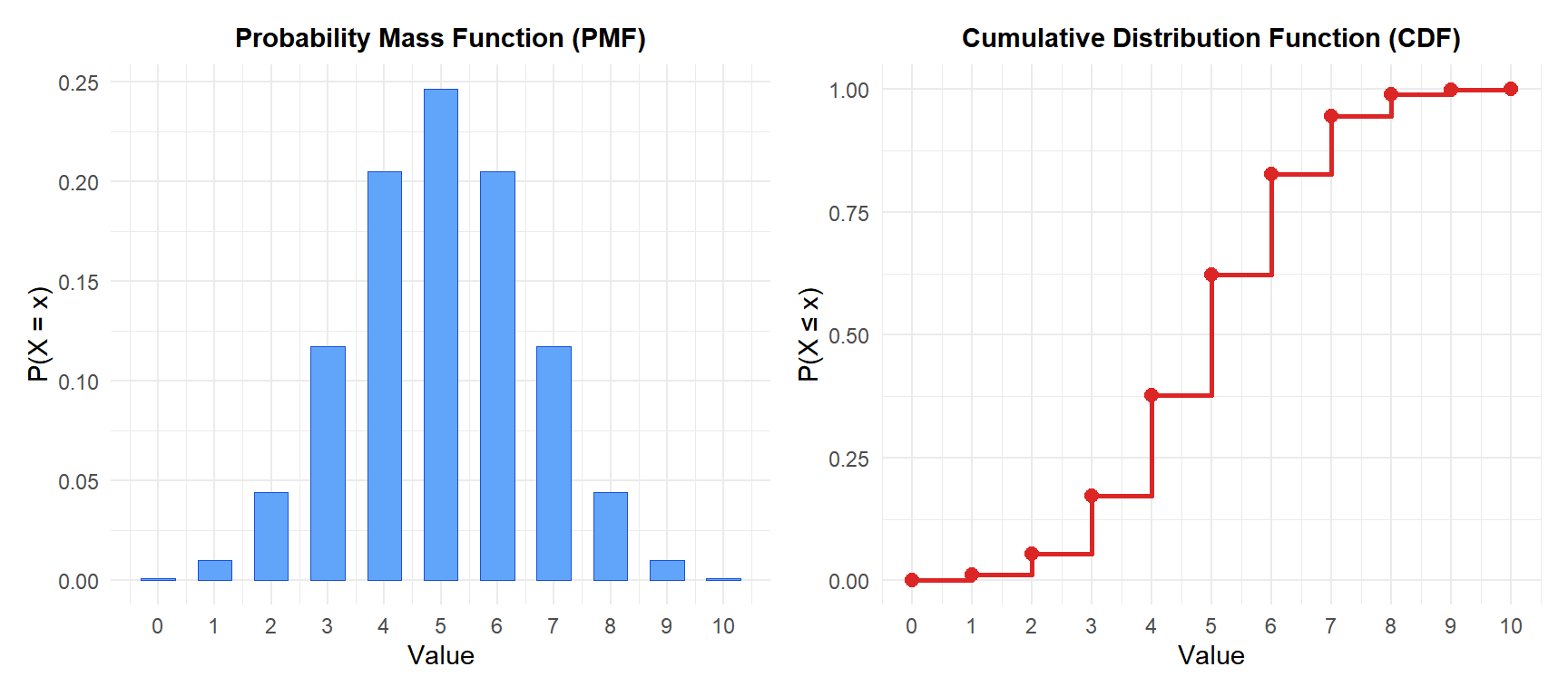
Figure 1: PMF (left) and CDF (right) of a Binomial(10, 0.5) distribution
A factory produces batches of 10 items. Each item is defective with probability 0.3, independently. The number of defective items (X \sim \text{Binomial}(10, 0.3)).
- \(P(X = 0) = 0.028\): probability of no defective items.
- \(P(X = 2) = 0.233\): most likely outcome.
- \(P(X \leq 3) = F(3) = 0.650\): 65% of batches have 3 or fewer defects.

Continuous random variables
A random variable is continuous when it can take any value within an interval (or union of intervals). Measurements like time, temperature, or weight are naturally continuous.
Probability density function (PDF)
For continuous variables, individual values have probability zero. Instead, probabilities are defined over intervals through the probability density function \(f(x)\):
\[ P(a \leq X \leq b) = \int_{a}^{b} f(x)\, dx, \quad \text{with } \int_{-\infty}^{\infty} f(x)\, dx = 1 \text{ and } f(x) \geq 0 \]
The PDF itself is not a probability: \(f(x)\) can exceed 1. It is a density, and only its integral over an interval gives a probability.
Cumulative distribution function (CDF)
The CDF for a continuous random variable is:
\[F(x) = P(X \leq x) = \int_{-\infty}^{x} f(t)\, dt\]
Unlike the discrete case, the continuous CDF is a smooth, non-decreasing function. The relationship between PDF and CDF is:
\[f(x) = \frac{d}{dx} F(x)\]
The PDF is the derivative of the CDF.
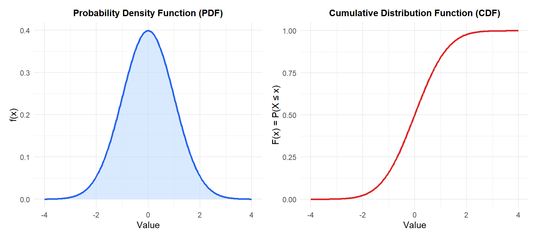
Figure 2: PDF (left) and CDF (right) of a standard normal distribution N(0,1)
⚠️ For continuous variables, P(X = x) = 0 always
This is the most common source of confusion when moving from discrete to continuous. For a continuous random variable, the probability of taking any single exact value is zero:
\[P(X = 2.5) = \int_{2.5}^{2.5} f(x)\, dx = 0\]
This does not mean the value is impossible. It means that in a continuous distribution, probabilities only make sense over intervals, not at individual points. As a consequence, for continuous variables \(P(X \leq x) = P(X < x)\): the distinction between strict and non-strict inequalities disappears.
Properties of the CDF
The CDF \(F(x)\) always satisfies these properties, whether the variable is discrete or continuous:
- \(\lim_{x \to -\infty} F(x) = 0\) and \(\lim_{x \to +\infty} F(x) = 1\).
- \(F\) is non-decreasing: if \(a < b\) then \(F(a) \leq F(b)\).
- \(F\) is right-continuous: \(\lim_{h \to 0^+} F(x+h) = F(x)\).
- \(P(a < X \leq b) = F(b) - F(a)\).
The CDF is the universal language for describing any random variable, discrete or continuous.
Mixed random variables
Some random variables are neither purely discrete nor purely continuous. A mixed random variable has a distribution with both a discrete component (positive probability at specific points) and a continuous component (a density over an interval).
An insurance policy pays nothing if no claim is filed, and a continuous positive amount otherwise. Let (X) be the claim amount:
- \(P(X = 0) = 0.6\): 60% of policyholders file no claim (discrete mass at zero).
- For \(X > 0\): \(X\) follows an exponential distribution (continuous component).
This is a mixed random variable: it has a point mass at 0 and a continuous density for positive values. Its CDF has a jump of 0.6 at zero, then rises smoothly for positive values.
💡 Which type do you have?

