Marginal probability density function
The marginal distribution of a variable is what you get when you look at that variable alone, ignoring all information about the other. It is obtained by summing (discrete) or integrating (continuous) the joint distribution over all possible values of the other variable.
Definition
Given the joint distribution of two random variables \((X, Y)\), the marginal distributions are the individual distributions of \(X\) and \(Y\) obtained by collapsing the joint distribution along one axis.
For continuous variables, the marginal PDFs are:
\[ f_X(x) = \int_{-\infty}^{\infty} f_{X,Y}(x,y)\, dy \qquad f_Y(y) = \int_{-\infty}^{\infty} f_{X,Y}(x,y)\, dx \]
For discrete variables, the marginal PMFs are obtained by summing over rows or columns of the joint table:
\[p_X(x) = \sum_{y} p_{X,Y}(x,y) \qquad p_Y(y) = \sum_{x} p_{X,Y}(x,y)\]
The name “marginal” comes from the practice of writing these sums in the margins of a joint probability table.
Discrete case: marginals from a joint table
Using the exercise and health score example from the previous sections:
| \(Y=1\) | \(Y=2\) | \(Y=3\) | \(p_X(x)\) | |
|---|---|---|---|---|
| \(X=0\) | 0.15 | 0.10 | 0.05 | 0.30 |
| \(X=1\) | 0.05 | 0.20 | 0.15 | 0.40 |
| \(X=2\) | 0.02 | 0.08 | 0.20 | 0.30 |
| \(p_Y(y)\) | 0.22 | 0.38 | 0.40 | 1.00 |
The marginal of \(X\) is the row totals: \(P(X=0) = 0.30\), \(P(X=1) = 0.40\), \(P(X=2) = 0.30\).
The marginal of \(Y\) is the column totals: \(P(Y=1) = 0.22\), \(P(Y=2) = 0.38\), \(P(Y=3) = 0.40\).
Each marginal is a valid PMF on its own: non-negative and sums to 1.
⚠️ Marginal vs conditional: a critical difference
These two concepts are frequently confused:
- The marginal \(p_X(x)\) ignores \(Y\) entirely. It is the distribution of \(X\) in the full population.
- The conditional \(P(X = x \mid Y = y)\) fixes \(Y\) at a specific value and looks at \(X\) within that subgroup.
From the table: \(P(X = 0) = 0.30\) (marginal), but \(P(X = 0 \mid Y = 1) = 0.15/0.22 \approx 0.68\) (conditional on poor health). They answer very different questions.
Continuous case: computing the marginal PDF
Suppose the joint PDF of \(X\) and \(Y\) is:
\[f_{X,Y}(x,y) = e^{-(x+y)}, \quad x \geq 0,\ y \geq 0\]
First, verify this is a valid joint PDF:
\[\int_0^\infty \int_0^\infty e^{-(x+y)}\, dy\, dx = \int_0^\infty e^{-x}\left[\int_0^\infty e^{-y}\, dy\right] dx = \int_0^\infty e^{-x} \cdot 1\, dx = 1 \checkmark\]
The marginal PDF of \(X\) is obtained by integrating out \(Y\):
\[f_X(x) = \int_0^\infty e^{-(x+y)}\, dy = e^{-x} \int_0^\infty e^{-y}\, dy = e^{-x} \cdot 1 = e^{-x}, \quad x \geq 0\]
So \(X \sim \text{Exponential}(1)\), with mean 1. By symmetry, \(Y\) has the same marginal distribution.
Note also that \(f_{X,Y}(x,y) = e^{-x} \cdot e^{-y} = f_X(x) \cdot f_Y(y)\), which confirms that \(X\) and \(Y\) are independent.
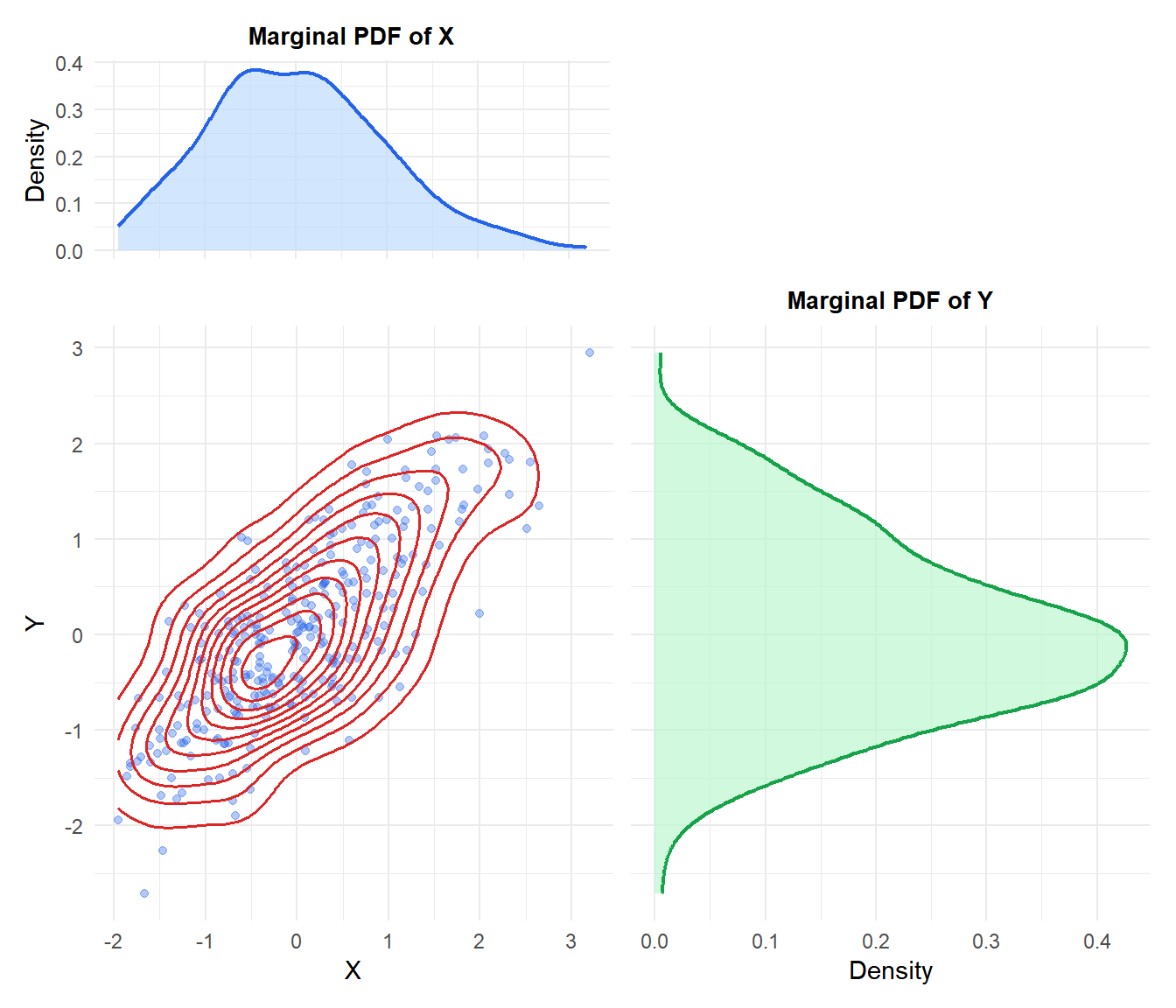
Figure 1: Joint distribution of two correlated variables (center) with their marginal PDFs projected onto each axis (top and right panels)
Key properties
- Each marginal is a valid PDF (or PMF): non-negative and integrates (or sums) to 1.
- The marginals do not uniquely determine the joint distribution: many different joint distributions can have the same marginals.
- If \(X\) and \(Y\) are independent, the joint distribution equals the product of the marginals: \(f_{X,Y}(x,y) = f_X(x) \cdot f_Y(y)\). The converse is also true.
Two very different joint distributions can share the same marginals. Suppose both \((X, Y)\) have marginals \(X \sim \text{Uniform}(0,1)\) and \(Y \sim \text{Uniform}(0,1)\). One joint could be the independent product (uniform on the unit square), and another could concentrate probability along the diagonal \(Y = X\). Both have identical marginals but completely different dependence structures. The marginals alone never tell you how the variables co-vary.
💡 How marginals relate to everything else
- Conditional PDF: divide the joint by the marginal of the conditioning variable.
- Independence: check whether the joint equals the product of marginals.
- Covariance: computed from the joint distribution, but the marginals give the individual means and variances needed in the formula.

