Joint probability density function
The joint probability density function (joint PDF) of two continuous random variables describes how probability is distributed across all possible pairs of values. Like the univariate PDF, it does not give probabilities directly: probabilities are obtained by integrating over a region of the plane.
Definition
A function \(f_{X,Y}(x,y)\) is the joint PDF of two continuous random variables \(X\) and \(Y\) if:
\[ P(a \leq X \leq b,\ c \leq Y \leq d) = \int_{a}^{b} \int_{c}^{d} f_{X,Y}(x,y)\, dy\, dx \]
To be a valid joint PDF, \(f_{X,Y}\) must satisfy:
- \(f_{X,Y}(x,y) \geq 0\) for all \((x,y)\).
- \(\int_{-\infty}^{\infty}\int_{-\infty}^{\infty} f_{X,Y}(x,y)\, dy\, dx = 1\).
The probability of any region \(A\) in the plane is the volume under the surface \(f_{X,Y}\) above \(A\).
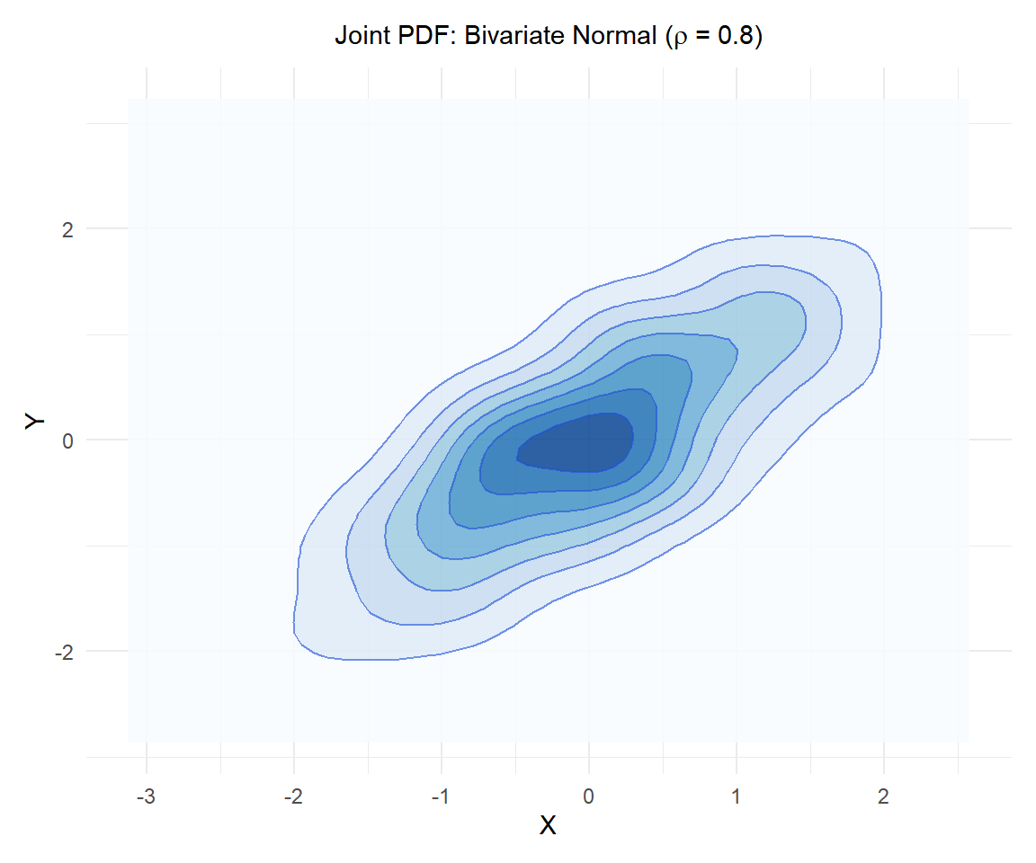
Figure 1: Joint PDF of a bivariate normal with correlation 0.8: the level curves show regions of equal density
The innermost ellipses correspond to the regions of highest density. The diagonal orientation reflects the positive correlation between \(X\) and \(Y\): when \(X\) is large, \(Y\) tends to be large as well.
Relationship with the joint distribution function
The joint PDF and the joint CDF \(F_{X,Y}(x,y)\) are related by:
\[F_{X,Y}(x,y) = \int_{-\infty}^{x} \int_{-\infty}^{y} f_{X,Y}(x', y')\, dy'\, dx'\]
The joint PDF is recovered by differentiating the joint CDF:
\[f_{X,Y}(x,y) = \frac{\partial^2 F_{X,Y}(x,y)}{\partial x\, \partial y}\]
Marginal densities
The marginal density of each variable is obtained by integrating the joint PDF over the other variable:
\[f_X(x) = \int_{-\infty}^{\infty} f_{X,Y}(x,y)\, dy \qquad f_Y(y) = \int_{-\infty}^{\infty} f_{X,Y}(x,y)\, dx\]
The marginal densities describe the behavior of each variable separately, ignoring the value of the other.
If ((X, Y)) follows a bivariate normal distribution with means (\mu_X), (\mu_Y), variances (\sigma_X^2), (\sigma_Y^2) and correlation (\rho), the marginal densities are:
\[f_X(x) = \frac{1}{\sigma_X\sqrt{2\pi}} e^{-\frac{(x-\mu_X)^2}{2\sigma_X^2}}, \qquad f_Y(y) = \frac{1}{\sigma_Y\sqrt{2\pi}} e^{-\frac{(y-\mu_Y)^2}{2\sigma_Y^2}}\]
Each variable separately follows a normal distribution, regardless of the value of \(\rho\). This is a special property of the bivariate normal distribution.
Independence
\(X\) and \(Y\) are independent if and only if their joint PDF factorizes:
\[f_{X,Y}(x,y) = f_X(x) \cdot f_Y(y)\]
In this case, the behavior of one variable provides no information about the other.
⚠️ Zero correlation does not imply independence in general
For the bivariate normal distribution, (\rho = 0) does imply independence. But this is an exception, not the rule. For most joint distributions, zero covariance does not imply independence: dependence can be non-linear and covariance does not capture it. Always verify the factorization of the joint PDF, not just the correlation coefficient.
Conditional density
The conditional density of \(Y\) given \(X = x\) is:
\[f_{Y|X}(y \mid x) = \frac{f_{X,Y}(x,y)}{f_X(x)}\]
It describes the distribution of \(Y\) when the value of \(X\) is fixed. For the bivariate normal, the conditional distribution of \(Y\) given \(X = x\) is also normal:
\[Y \mid X = x \sim \mathcal{N}\!\left(\mu_Y + \rho\frac{\sigma_Y}{\sigma_X}(x - \mu_X),\ \sigma_Y^2(1-\rho^2)\right)\]
The conditional mean is linear in \(x\) and the conditional variance is smaller than the marginal variance when \(|\rho| > 0\).
💡 Joint PDF vs marginal PDF: when to use each

