Cumulative distribution function
The cumulative distribution function (CDF) gives the probability that a random variable takes a value less than or equal to a specific point. It works for any type of random variable and is the foundation for calculating probabilities, generating random samples, and defining quantiles.
Definition
The cumulative distribution function of a random variable \(X\) is defined as:
ℹ️ CDF of a random variable
\[ F(x) = P(X \leq x), \quad \text{for all } x \in \mathbb{R} \]
The CDF accumulates probability from \(-\infty\) up to \(x\). It is defined for any real number \(x\), not just the values where \(X\) has positive probability.
Properties of the CDF
Every CDF, regardless of the type of random variable, satisfies the following properties:
- Limits: \(\lim_{x \to -\infty} F(x) = 0\) and \(\lim_{x \to +\infty} F(x) = 1\).
- Non-decreasing: if \(a < b\) then \(F(a) \leq F(b)\).
- Bounded: \(0 \leq F(x) \leq 1\) for all \(x\).
- Right-continuous: \(\lim_{h \to 0^+} F(x+h) = F(x)\).
- Interval probability: \(P(a < X \leq b) = F(b) - F(a)\).
The last property is the most practically useful: you can compute the probability of any interval using just two evaluations of the CDF.
CDF for discrete random variables
For a discrete random variable with possible values \(x_1 < x_2 < \cdots\) and probabilities \(p_i = P(X = x_i)\), the CDF is:
ℹ️ CDF for discrete variables
\[ F(x) = \sum_{x_i \leq x} p_i \]
The CDF of a discrete variable is a step function: it stays flat between consecutive values and jumps at each \(x_i\) by exactly \(p_i\).
Flip a fair coin twice. Let (X) = number of heads. The PMF is:
- \(P(X = 0) = 0.25\), \(P(X = 1) = 0.50\), \(P(X = 2) = 0.25\)
The CDF is:
- \(F(x) = 0\) for \(x < 0\)
- \(F(x) = 0.25\) for \(0 \leq x < 1\)
- \(F(x) = 0.75\) for \(1 \leq x < 2\)
- \(F(x) = 1.00\) for \(x \geq 2\)
So \(P(X \leq 1) = 0.75\): there is a 75% chance of getting at most one head.
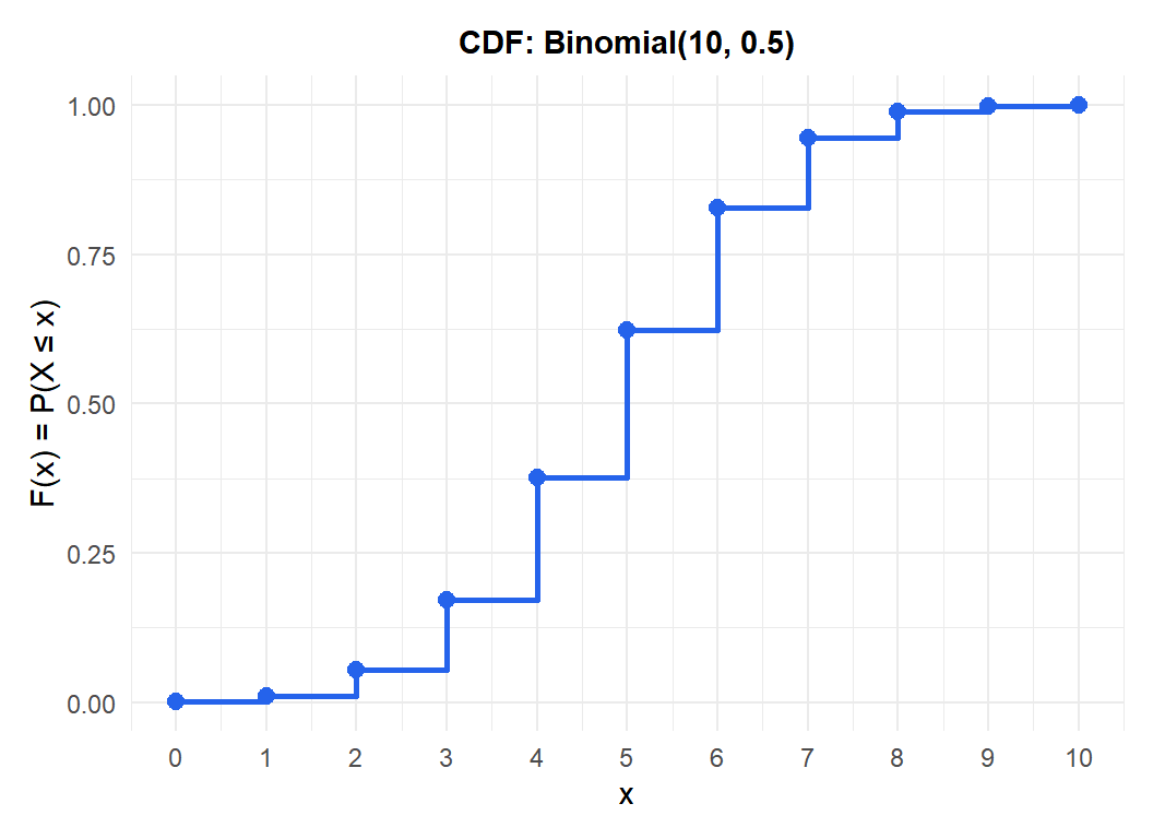
Figure 1: CDF of a Binomial(10, 0.5) distribution: a step function that jumps at each possible value
⚠️ In discrete variables, P(X < x) ≠ P(X ≤ x)
For discrete random variables, the strict and non-strict inequalities are not the same:
\[P(X < 2) = F(1) = 0.75 \neq P(X \leq 2) = F(2) = 1.00\]
The difference is exactly \(P(X = 2) = 0.25\). This distinction disappears for continuous variables, where \(P(X = x) = 0\) for any single point, but for discrete variables it matters and is a common source of errors in exam calculations.
CDF for continuous random variables
For a continuous random variable with probability density function \(f(x)\), the CDF is:
ℹ️ CDF for continuous variables
\[ F(x) = \int_{-\infty}^{x} f(t)\, dt \]
The CDF is a smooth, non-decreasing curve from 0 to 1. The relationship between PDF and CDF is:
\[f(x) = \frac{d}{dx} F(x)\]
The PDF is the derivative of the CDF, and the CDF is the integral of the PDF.
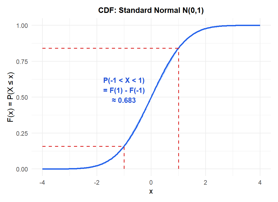
Figure 2: CDF of N(0,1): the shaded area between -1 and 1 equals F(1) - F(-1) ≈ 0.683
A web server’s response time follows an exponential distribution with mean 200 ms, so (\lambda = 1/200).
The CDF is \(F(x) = 1 - e^{-x/200}\) for \(x > 0\).
- Probability of responding in under 100 ms: \(F(100) = 1 - e^{-0.5} \approx 0.393\)
- Probability of responding in under 500 ms: \(F(500) = 1 - e^{-2.5} \approx 0.918\)
- Probability of taking between 100 and 500 ms: \(F(500) - F(100) \approx 0.918 - 0.393 = 0.525\)
All three answers come from two evaluations of the CDF.
The inverse CDF: quantile function
The quantile function (or inverse CDF) is \(F^{-1}(p)\): it gives the value \(x\) such that \(F(x) = p\).
\[Q(p) = F^{-1}(p) = \inf\{x : F(x) \geq p\}\]
This is how percentiles and quantiles are defined formally. The median is \(Q(0.5)\), the first quartile is \(Q(0.25)\), and so on.
💡 The quantile function is essential for simulation
CDF for mixed random variables
Mixed random variables have a CDF that combines jumps (from the discrete component) with smooth sections (from the continuous component). The CDF is still right-continuous and non-decreasing, but it is neither a pure step function nor a smooth curve.
An insurance policy pays zero with probability 0.6 (no claim filed) and a positive amount following an exponential distribution otherwise. The CDF is:
- \(F(0) = 0.6\) (jump of 0.6 at zero)
- \(F(x) = 0.6 + 0.4(1 - e^{-\lambda x})\) for \(x > 0\) (smooth exponential rise)
The CDF starts at 0, jumps to 0.6 at \(x = 0\), then increases smoothly to 1.

