Bidimensional random variables

When two random variables are measured on the same individual or experiment, you need tools that describe their joint behavior, not just each one separately. Bidimensional random variables provide exactly that: a framework for studying how two variables relate, depend on, or influence each other.

Definition

A bidimensional random variable is a pair \((X, Y)\) of random variables defined on the same probability space:

Each outcome \(\omega \in \Omega\) is assigned a pair of real numbers \((X(\omega), Y(\omega))\). The full probabilistic behavior of the pair is described by its joint distribution.

Joint distribution

The joint distribution describes the probability of \((X, Y)\) taking specific values simultaneously.

For discrete variables, the joint probability mass function is:

\[p_{X,Y}(x, y) = P(X = x,\ Y = y)\]

For continuous variables, the joint probability density function \(f_{X,Y}(x, y)\) satisfies:

\[P((X,Y) \in A) = \iint_A f_{X,Y}(x, y)\, dx\, dy\]

In both cases the joint distribution must satisfy non-negativity and normalization (the total probability sums or integrates to 1).

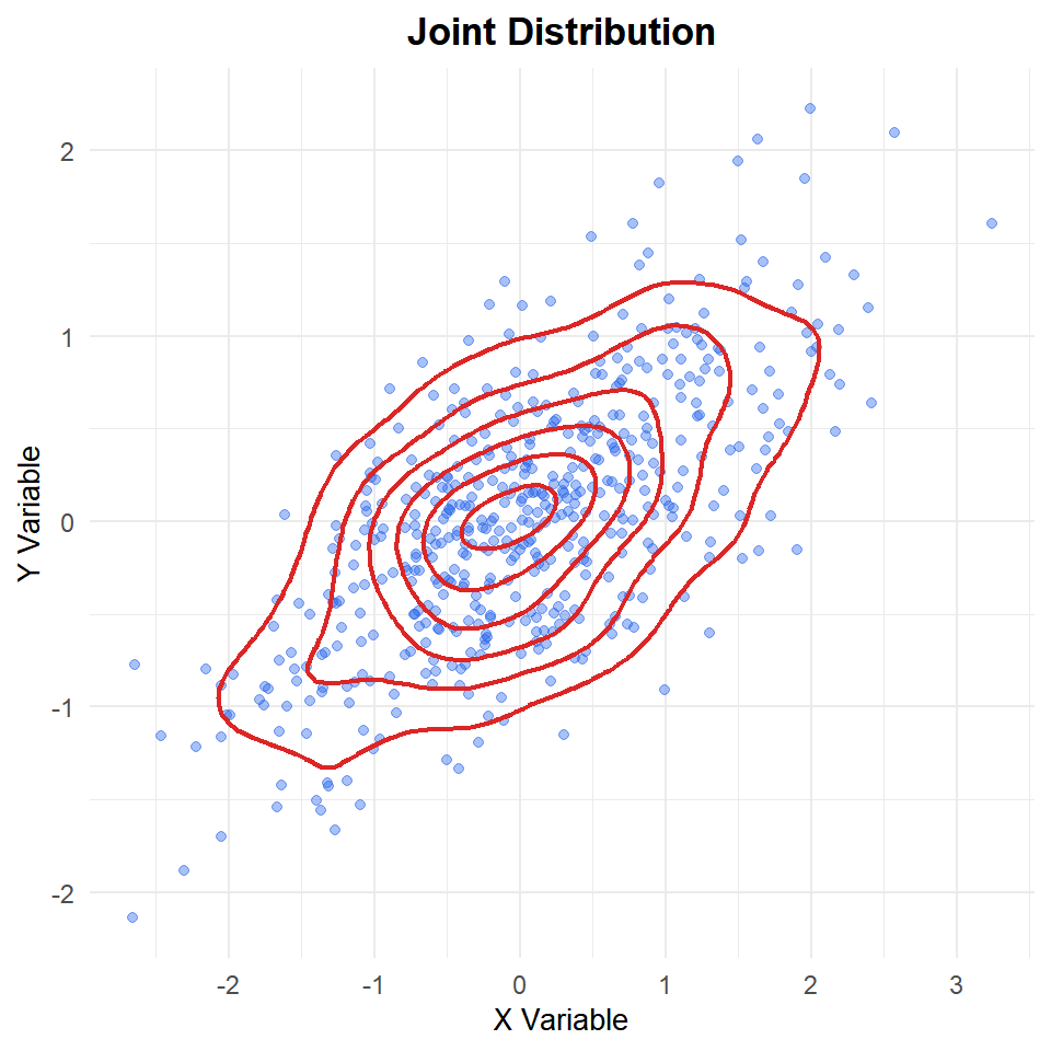
Figure 1: Joint distribution of two correlated continuous variables: each point is one observation, contours show regions of equal density

Joint distribution table: discrete case

A survey records the number of hours of exercise per week (\(X\)) and the self-reported health score (\(Y\), from 1 to 3) for a sample of individuals. The joint PMF is:

	\(Y=1\) (poor)	\(Y=2\) (fair)	\(Y=3\) (good)	\(p_X(x)\)
\(X=0\) (sedentary)	0.15	0.10	0.05	0.30
\(X=1\) (moderate)	0.05	0.20	0.15	0.40
\(X=2\) (active)	0.02	0.08	0.20	0.30
\(p_Y(y)\)	0.22	0.38	0.40	1.00

The row sums give the marginal distribution of \(X\); the column sums give the marginal distribution of \(Y\).

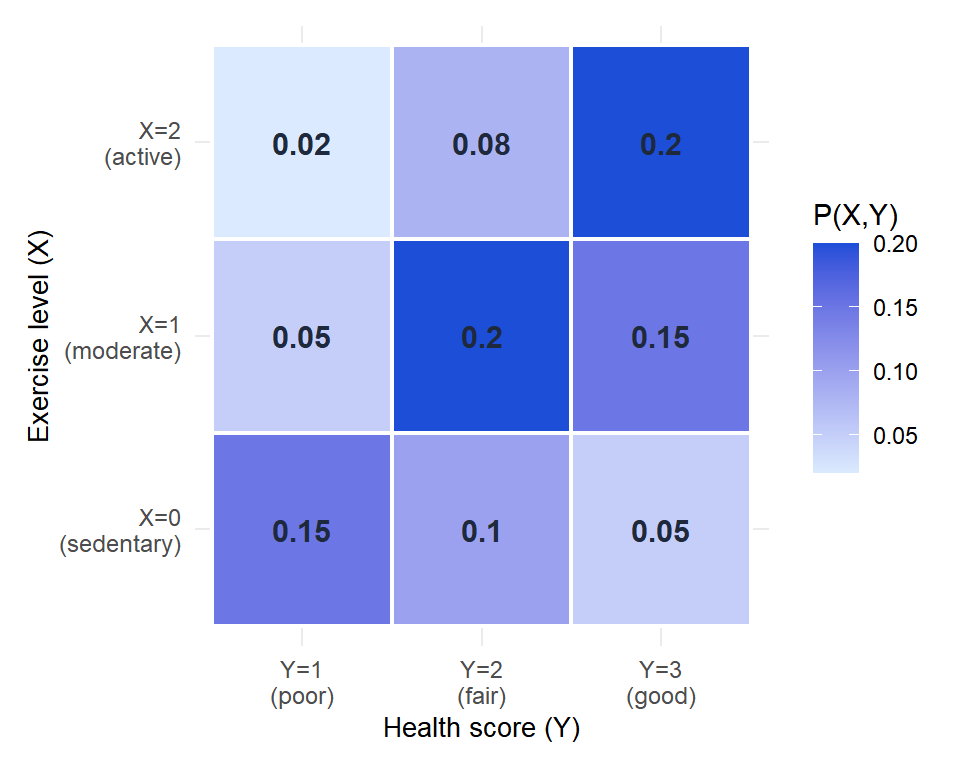
Figure 2: Joint PMF as a heatmap: darker cells have higher joint probability

Marginal distributions

The marginal distribution of \(X\) is obtained by summing (or integrating) the joint distribution over all values of \(Y\), and vice versa.

For discrete variables:

\[p_X(x) = \sum_{y} p_{X,Y}(x, y) \qquad p_Y(y) = \sum_{x} p_{X,Y}(x, y)\]

For continuous variables:

\[f_X(x) = \int_{-\infty}^{\infty} f_{X,Y}(x, y)\, dy \qquad f_Y(y) = \int_{-\infty}^{\infty} f_{X,Y}(x, y)\, dx\]

Using the table above, the marginal distribution of \(X\) is:

• \(P(X=0) = 0.15 + 0.10 + 0.05 = 0.30\)
• \(P(X=1) = 0.05 + 0.20 + 0.15 = 0.40\)
• \(P(X=2) = 0.02 + 0.08 + 0.20 = 0.30\)

These are the row totals. The marginal of \(Y\) is computed from column totals in the same way.

Conditional distributions

The conditional distribution of \(X\) given \(Y = y\) describes how \(X\) behaves when we fix the value of \(Y\). For discrete variables:

\[P(X = x \mid Y = y) = \frac{P(X = x,\ Y = y)}{P(Y = y)}\]

For continuous variables:

\[f_{X \mid Y}(x \mid y) = \frac{f_{X,Y}(x, y)}{f_Y(y)}\]

Conditional distribution: exercise given poor health

Using the table above, what is the distribution of exercise level given that a person has poor health ((Y = 1))?

\[P(X=0 \mid Y=1) = \frac{0.15}{0.22} \approx 0.682\] \[P(X=1 \mid Y=1) = \frac{0.05}{0.22} \approx 0.227\] \[P(X=2 \mid Y=1) = \frac{0.02}{0.22} \approx 0.091\]

Among people with poor health, 68% are sedentary and only 9% are active. This is the conditional distribution of \(X\) given \(Y = 1\).

Independence

\(X\) and \(Y\) are independent if and only if their joint distribution factorizes into the product of the marginal distributions:

\[p_{X,Y}(x, y) = p_X(x) \cdot p_Y(y) \quad \text{(discrete)}\]

\[f_{X,Y}(x, y) = f_X(x) \cdot f_Y(y) \quad \text{(continuous)}\]

In practice, to check independence in a discrete table: verify that every cell equals the product of its row and column marginals. One cell that violates this is enough to conclude dependence.

For the exercise/health table, checking cell \((X=0, Y=3)\):

\[p_X(0) \cdot p_Y(3) = 0.30 \times 0.40 = 0.12 \neq 0.05 = p_{X,Y}(0,3)\]

The variables are not independent: exercise level and health score are associated.