Law of total probability
The law of total probability expresses the probability of an event as a weighted average of its conditional probabilities across all possible scenarios. It is the tool that turns a complex, hard-to-compute probability into a sum of simpler conditional ones.
Definition
Let \(A_1, A_2, \ldots, A_n\) be a partition of the sample space \(\Omega\): the events are mutually exclusive (\(A_i \cap A_j = \emptyset\) for \(i \neq j\)) and exhaustive (\(A_1 \cup A_2 \cup \cdots \cup A_n = \Omega\)). For any event \(B\):
\[P(B) = \sum_{i=1}^{n} P(B \mid A_i) \cdot P(A_i)\]
The intuition: \(B\) can only happen via one of the scenarios \(A_i\). The total probability of \(B\) is the sum of the probabilities of \(B\) happening through each scenario, weighted by how likely each scenario is.
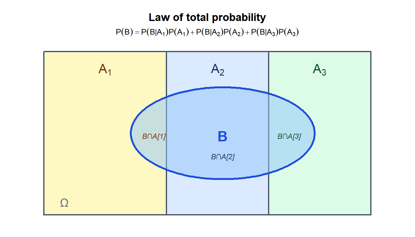
The diagram shows \(B\) cutting across all three partition cells. The total probability of \(B\) is the sum of the three shaded overlaps, each weighted by the probability of its partition cell.
⚠️ The partition must be exhaustive and mutually exclusive
The law only works when \(A_1, \ldots, A_n\) truly cover every possible outcome and do not overlap. Two common mistakes:
- Forgetting a scenario: if a factory has three suppliers but you only condition on two, the formula gives the wrong answer.
- Overlapping categories: if a patient can belong to two disease categories simultaneously, \(A_i\) are not mutually exclusive and the formula overcounts.
Always verify: do the \(A_i\) add up to 1? \(\sum_i P(A_i) = 1\) is a necessary check.
Two-scenario case
The simplest partition is \(\{A, A^c\}\). The law reduces to:
\[P(B) = P(B \mid A) \cdot P(A) + P(B \mid A^c) \cdot P(A^c)\]
This is the form most often seen in medical testing and classification problems.
A disease affects 2% of the population (\(P(D) = 0.02\)). A test has:
- Sensitivity: \(P(+ \mid D) = 0.95\).
- Specificity: \(P(- \mid D^c) = 0.90\), so \(P(+ \mid D^c) = 0.10\).
What fraction of the population tests positive?
\[P(+) = P(+ \mid D) \cdot P(D) + P(+ \mid D^c) \cdot P(D^c)\] \[= 0.95 \times 0.02 + 0.10 \times 0.98 = 0.019 + 0.098 = 0.117\]
About 11.7% of the population tests positive, even though only 2% actually has the disease. This is the denominator needed to apply Bayes theorem and find \(P(D \mid +)\).
Three or more scenarios
A company sources components from three suppliers:
- Supplier A provides 50% of components, with a 3% defect rate.
- Supplier B provides 30%, with a 5% defect rate.
- Supplier C provides 20%, with a 8% defect rate.
What is the overall defect rate?
\[P(\text{defect}) = 0.03 \times 0.50 + 0.05 \times 0.30 + 0.08 \times 0.20\] \[= 0.015 + 0.015 + 0.016 = 0.046\]
The overall defect rate is 4.6%. Note that supplier C contributes 0.016 to the total despite only providing 20% of components, because its defect rate is much higher.
A subscription service has three customer segments:
- Premium users (25% of base): 5% monthly churn rate.
- Standard users (50% of base): 15% monthly churn rate.
- Free users (25% of base): 40% monthly churn rate.
Overall monthly churn rate:
\[P(\text{churn}) = 0.05 \times 0.25 + 0.15 \times 0.50 + 0.40 \times 0.25\] \[= 0.0125 + 0.075 + 0.10 = 0.1875\]
18.75% of all users churn each month. The free tier alone accounts for \(0.10/0.1875 \approx 53\%\) of all churned users despite being only 25% of the base.
Connection to Bayes theorem
The law of total probability is the denominator in Bayes theorem. Combining both:
\[P(A_i \mid B) = \frac{P(B \mid A_i) \cdot P(A_i)}{P(B)} = \frac{P(B \mid A_i) \cdot P(A_i)}{\displaystyle\sum_{j=1}^{n} P(B \mid A_j) \cdot P(A_j)}\]
The law of total probability computes \(P(B)\) so that Bayes theorem can update the probabilities of each scenario \(A_i\) after observing \(B\).
Using the supplier example above, a defective component is found. What is the probability it came from supplier C?
\[P(C \mid \text{defect}) = \frac{P(\text{defect} \mid C) \cdot P(C)}{P(\text{defect})} = \frac{0.08 \times 0.20}{0.046} = \frac{0.016}{0.046} \approx 0.348\]
Even though C provides only 20% of components, it is responsible for about 35% of defects. The law of total probability (0.046) is the key ingredient that makes this calculation possible.
💡 When to use the law of total probability
Use it when:
- \(P(B)\) is hard to compute directly but \(P(B \mid A_i)\) is known for each scenario.
- You have a mixture of subpopulations with different rates (defect rates by supplier, churn by segment, test sensitivity by disease status).
- You need the denominator for Bayes theorem.
The law is essentially a weighted average: the overall probability of \(B\) is the average of the conditional probabilities, weighted by how likely each condition is.

