Incompatible (Disjoint) Events
Two events are incompatible (or disjoint) when they cannot both occur in the same trial. Their intersection is empty, and their probabilities add directly. This is the simplest case of the addition rule and appears naturally whenever outcomes fall into non-overlapping categories.
Definition
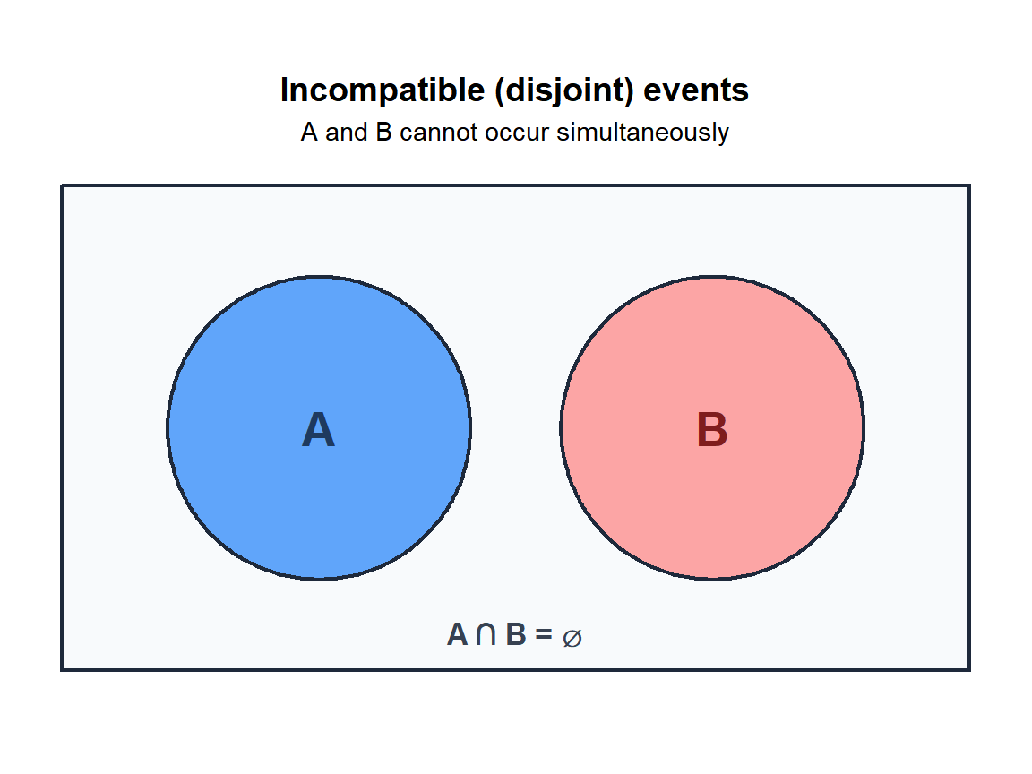
Events \(A\) and \(B\) are incompatible (also called mutually exclusive or disjoint) if they share no outcomes:
\[A \cap B = \emptyset \quad \Longleftrightarrow \quad P(A \cap B) = 0\]
When \(A\) and \(B\) are disjoint, the addition rule simplifies to:
\[P(A \cup B) = P(A) + P(B)\]
For any collection of pairwise disjoint events \(A_1, A_2, \ldots, A_n\):
\[P(A_1 \cup A_2 \cup \cdots \cup A_n) = P(A_1) + P(A_2) + \cdots + P(A_n)\]
This is the countable additivity property, one of the three Kolmogorov axioms of probability.
Examples
Example 1: customer classification
An e-commerce platform classifies each order into exactly one status category:
- \(A\) = order delivered on time
- \(B\) = order delayed
- \(C\) = order cancelled
These three events are pairwise disjoint: an order cannot be in two categories simultaneously. If \(P(A) = 0.78\), \(P(B) = 0.15\), and \(P(C) = 0.07\):
\[P(A \cup B \cup C) = 0.78 + 0.15 + 0.07 = 1.00\]
They are also exhaustive: every order falls into exactly one category. Together they form a partition of the sample space.
\[P(\text{not delivered on time}) = P(B \cup C) = P(B) + P(C) = 0.15 + 0.07 = 0.22\]
Example 2: insurance claim types
An insurance company models claims by type. A single claim is classified as one of:
- \(A\) = property damage only: \(P(A) = 0.45\)
- \(B\) = personal injury only: \(P(B) = 0.30\)
- \(C\) = both property and personal: \(P(C) = 0.25\)
Here \(A\) and \(B\) are disjoint (a claim in category \(A\) is property only, explicitly excluding injury). But \(A\) and \(C\) are not disjoint: both involve property damage.
\[P(A \cup B) = P(A) + P(B) = 0.45 + 0.30 = 0.75\]
\[P(\text{involves property}) = P(A) + P(C) = 0.45 + 0.25 = 0.70\]
Note: the second calculation uses addition without the overlap correction because \(A\) and \(C\) are defined to be mutually exclusive in this classification system.
Example 3: defect categories in manufacturing
A component inspection classifies each defective item into exactly one defect type:
- \(D_1\) = dimensional error: \(P(D_1) = 0.06\)
- \(D_2\) = surface defect: \(P(D_2) = 0.03\)
- \(D_3\) = material flaw: \(P(D_3) = 0.01\)
These are defined as mutually exclusive (each item is assigned to its primary defect type). The total defect rate is:
\[P(\text{defective}) = P(D_1) + P(D_2) + P(D_3) = 0.06 + 0.03 + 0.01 = 0.10\]
10% of components have at least one defect. The addition works directly because the categories are disjoint by construction.
A hospital emergency department tracks patient triage levels: Critical (5%), Urgent (25%), Semi-urgent (40%), Non-urgent (30%). These are disjoint and exhaustive.
Probability of a patient needing immediate attention (Critical or Urgent):
\[P(\text{immediate}) = P(\text{Critical}) + P(\text{Urgent}) = 0.05 + 0.25 = 0.30\]
Probability of a patient not needing immediate attention:
\[P(\text{not immediate}) = 1 - 0.30 = 0.70\]
Or directly: \(0.40 + 0.30 = 0.70\). Both give the same answer because the four categories partition the space.
Disjoint vs independent: a critical distinction
⚠️ Disjoint events with positive probability are never independent
This is one of the most common confusions in probability. If \(A\) and \(B\) are disjoint and both have positive probability:
\[P(A \cap B) = 0 \neq P(A) \cdot P(B) > 0\]
So they cannot be independent. The reason is intuitive: if \(A\) and \(B\) cannot both happen, then knowing \(A\) occurred tells you immediately that \(B\) did not. That is the opposite of independence.
Examples that are disjoint but NOT independent:
- A machine produces exactly one item per cycle, classified as good or defective. “Good” and “defective” are disjoint; knowing one excludes the other completely.
- A patient is assigned to treatment A or treatment B (not both). The two assignments are disjoint; they give maximum information about each other.
The only way disjoint events can be independent is if at least one has probability zero, making independence a degenerate case.
The contrast:
- Disjoint: \(A\) and \(B\) cannot both occur. \(P(A \cap B) = 0\). Knowing one occurred tells you the other did not.
- Independent: \(A\) and \(B\) do not influence each other. \(P(A \cap B) = P(A) \cdot P(B)\). Knowing one occurred tells you nothing about the other.
💡 When to apply the simplified addition rule
\(P(A \cup B) = P(A) + P(B)\) is only valid when \(A\) and \(B\) are disjoint. Before using it, verify that the events truly cannot overlap. Common disjoint structures:
- Classification systems where each outcome falls into exactly one category.
- Competing causes of failure where a component can fail for one reason at a time.
- Exhaustive partitions of a population or sample space.
If there is any chance of overlap, use the full formula: \(P(A \cup B) = P(A) + P(B) - P(A \cap B)\).

