Bayes theorem
Bayes theorem tells you how to update a probability when new evidence arrives. It connects what you knew before (the prior) with what the data tells you (the likelihood) to produce an updated belief (the posterior). It is the mathematical foundation of rational reasoning under uncertainty.
Definition
For two events \(A\) and \(B\) with \(P(B) > 0\):
\[P(A \mid B) = \frac{P(B \mid A) \cdot P(A)}{P(B)}\]
Each component has a name and a role:
| Term | Notation | Meaning |
|---|---|---|
| Prior | \(P(A)\) | Probability of \(A\) before observing \(B\) |
| Likelihood | \(P(B \mid A)\) | Probability of observing \(B\) if \(A\) is true |
| Posterior | \(P(A \mid B)\) | Updated probability of \(A\) after observing \(B\) |
| Marginal likelihood | \(P(B)\) | Total probability of observing \(B\) (normalizing constant) |
When the hypothesis space has multiple alternatives \(A_1, \ldots, A_n\) forming a partition, the denominator expands via the law of total probability:
\[P(A_i \mid B) = \frac{P(B \mid A_i) \cdot P(A_i)}{\displaystyle\sum_{j=1}^{n} P(B \mid A_j) \cdot P(A_j)}\]
Bayesian updating: from prior to posterior
The key insight of Bayes theorem is that it describes a process of belief updating. You start with a prior, observe evidence, and arrive at a posterior. The posterior from one observation becomes the prior for the next.
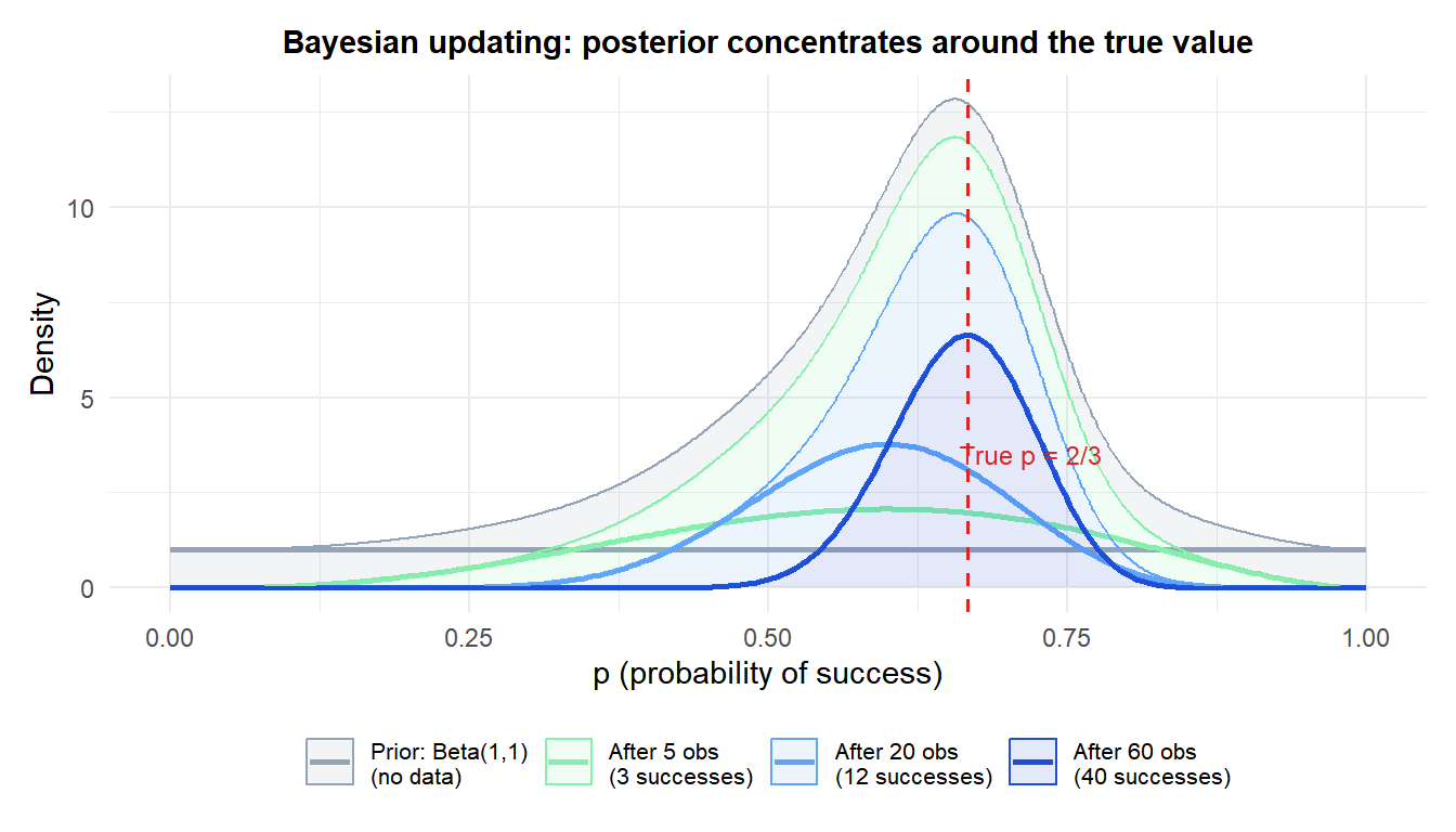
With a flat prior (all values of \(p\) equally plausible), each batch of observations shifts and narrows the posterior. After 60 observations, the distribution is tightly concentrated around the true value of \(2/3\).
Step-by-step examples
Example 1: medical diagnosis
A rare disease affects 0.5% of the population. A screening test has:
- Sensitivity: \(P(+ \mid D) = 0.92\)
- False positive rate: \(P(+ \mid D^c) = 0.04\)
A patient tests positive. What is the probability they have the disease?
Prior: \(P(D) = 0.005\), \(P(D^c) = 0.995\)
Marginal likelihood via law of total probability:
\[P(+) = 0.92 \times 0.005 + 0.04 \times 0.995 = 0.0046 + 0.0398 = 0.0444\]
Posterior:
\[P(D \mid +) = \frac{0.92 \times 0.005}{0.0444} = \frac{0.0046}{0.0444} \approx 0.104\]
Only 10.4% of people who test positive actually have the disease. The test is fairly accurate, but the disease is so rare that false positives dominate.
Out of 10,000 people:
- 50 have the disease. Of those, \(50 \times 0.92 = 46\) test positive (true positives).
- 9,950 are healthy. Of those, \(9950 \times 0.04 = 398\) test positive (false positives).
Total positives: \(46 + 398 = 444\).
\[P(D \mid +) = \frac{46}{444} \approx 0.104 \checkmark\]
Natural frequencies make the result intuitive: of 444 positive tests, only 46 are real cases.
Example 2: spam filter with multiple words
A spam filter starts with prior \(P(\text{spam}) = 0.30\). The word “urgent” appears in:
- 45% of spam emails: \(P(\text{urgent} \mid \text{spam}) = 0.45\)
- 3% of legitimate emails: \(P(\text{urgent} \mid \text{legit}) = 0.03\)
After observing “urgent”:
\[P(\text{urgent}) = 0.45 \times 0.30 + 0.03 \times 0.70 = 0.135 + 0.021 = 0.156\]
\[P(\text{spam} \mid \text{urgent}) = \frac{0.45 \times 0.30}{0.156} \approx 0.865\]
The posterior (86.5%) becomes the new prior for the next word. If the email also contains “winner”:
- \(P(\text{winner} \mid \text{spam}) = 0.60\), \(P(\text{winner} \mid \text{legit}) = 0.01\)
\[P(\text{spam} \mid \text{urgent, winner}) = \frac{0.60 \times 0.865}{0.60 \times 0.865 + 0.01 \times 0.135} \approx \frac{0.519}{0.519 + 0.00135} \approx 0.997\]
Near certainty of spam after just two suspicious words. This sequential updating is the core of Naive Bayes classifiers.
Example 3: three competing hypotheses
A quality analyst finds a defective component. It came from one of three suppliers:
- Supplier X provides 50% of parts, with a 2% defect rate.
- Supplier Y provides 30%, with a 5% defect rate.
- Supplier Z provides 20%, with a 8% defect rate.
Priors: \(P(X) = 0.50\), \(P(Y) = 0.30\), \(P(Z) = 0.20\)
Marginal likelihood:
\[P(\text{defect}) = 0.02 \times 0.50 + 0.05 \times 0.30 + 0.08 \times 0.20 = 0.010 + 0.015 + 0.016 = 0.041\]
Posteriors:
\[P(X \mid \text{defect}) = \frac{0.02 \times 0.50}{0.041} \approx 0.244\]
\[P(Y \mid \text{defect}) = \frac{0.05 \times 0.30}{0.041} \approx 0.366\]
\[P(Z \mid \text{defect}) = \frac{0.08 \times 0.20}{0.041} \approx 0.390\]
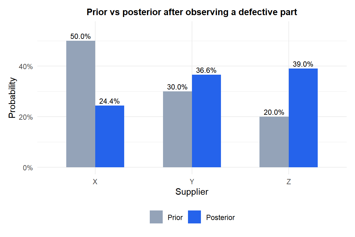
Supplier Z jumps from 20% prior to 39% posterior: even though it provides the fewest parts, its high defect rate makes it the most likely source of any given defect.
The prosecutor’s fallacy
⚠️ P(evidence | innocent) is not P(innocent | evidence)
The prosecutor’s fallacy is confusing the likelihood \(P(E \mid H)\) with the posterior \(P(H \mid E)\). A classic example:
- DNA evidence matches the suspect with probability \(P(\text{match} \mid \text{innocent}) = 1/1{,}000{,}000\).
- A prosecutor claims: “There is only a 1 in a million chance the suspect is innocent.”
This is wrong. \(P(\text{match} \mid \text{innocent})\) is not \(P(\text{innocent} \mid \text{match})\). The correct calculation requires the prior probability that the suspect is guilty, the size of the population, and the probability of a coincidental match. In a city of 1 million, one would expect one innocent person to also match the DNA profile. The posterior probability of innocence given a match could be 50%, not 1 in a million.
This error has contributed to wrongful convictions. Bayes theorem is the correct tool for evaluating forensic evidence.
Frequentist vs Bayesian interpretation
Bayes theorem itself is mathematically uncontroversial: it follows directly from the definition of conditional probability. The debate is about how to use it:
- Frequentists accept Bayes theorem as a probability rule but reject the idea of assigning prior probabilities to hypotheses (which they view as fixed, not random). They use it only when \(A\) is a random event with a well-defined frequency.
- Bayesians use Bayes theorem as the general rule for updating any degree of belief, including beliefs about fixed but unknown parameters. The prior encodes existing knowledge or assumptions, and the posterior summarizes what is known after seeing the data.
In practice, Bayesian methods are used in machine learning (Naive Bayes, Bayesian networks), clinical trial design, A/B testing, and any domain where incorporating prior knowledge is valuable.
💡 The three-step recipe for applying Bayes theorem
Every application of Bayes theorem follows the same structure:
- State the prior \(P(A)\): what do you believe before seeing the evidence?
- Specify the likelihood \(P(B \mid A)\): how probable is the evidence under each hypothesis?
- Compute the marginal likelihood \(P(B)\) using the law of total probability.
- Apply Bayes theorem to get the posterior \(P(A \mid B)\).
The posterior answers the question you actually care about. The likelihood answers the reverse question, which is often easier to measure (a lab can measure test sensitivity; a patient wants to know their risk).

