Newton's method and BFGS
Newton’s method uses second-order information (the Hessian matrix) to take curved steps toward the optimum, achieving quadratic convergence: the number of correct digits roughly doubles at each iteration. BFGS approximates the Hessian from gradient information alone, getting near-Newton convergence without the \(O(n^3)\) cost of inverting a dense matrix.
Newton’s method
Gradient descent uses only the gradient: it moves in the direction of steepest descent with a fixed step size. This ignores the curvature of \(f\): in directions where the function curves steeply, the step is too large and the algorithm oscillates; in flat directions, it is too small.
Newton’s method fits a local quadratic approximation to \(f\) at \(x_k\) using the second-order Taylor expansion:
\[f(x) \approx f(x_k) + \nabla f(x_k)^T(x - x_k) + \frac{1}{2}(x-x_k)^T \nabla^2 f(x_k)(x-x_k)\]
Minimizing this quadratic in \(x\) gives the Newton step:
\[x_{k+1} = x_k - \left[\nabla^2 f(x_k)\right]^{-1} \nabla f(x_k)\]
\[p_k = -H_k^{-1} g_k \qquad \text{where } H_k = \nabla^2 f(x_k),\; g_k = \nabla f(x_k)\]
The Hessian \(H_k\) scales the gradient by the local curvature: in steep directions (large eigenvalues of \(H_k\)) the step is small; in flat directions (small eigenvalues) the step is large. This automatically adapts the step size to the geometry of \(f\).
Quadratic convergence
Near a non-degenerate local minimum \(x^*\) where \(H^* = \nabla^2 f(x^*)\) is positive definite, Newton’s method converges quadratically:
\[\|x_{k+1} - x^*\| \leq C \|x_k - x^*\|^2\]
for some constant \(C > 0\). If the error at step \(k\) is \(\varepsilon\), the error at step \(k+1\) is roughly \(C\varepsilon^2\). This means the number of correct decimal digits doubles at each iteration: if you have 2 correct digits, the next step gives 4, then 8, then 16.
Compare with gradient descent’s linear convergence \(\|x_{k+1} - x^*\| \leq \rho \|x_k - x^*\|\) for some \(\rho < 1\): errors decrease by a constant factor, not squaring.
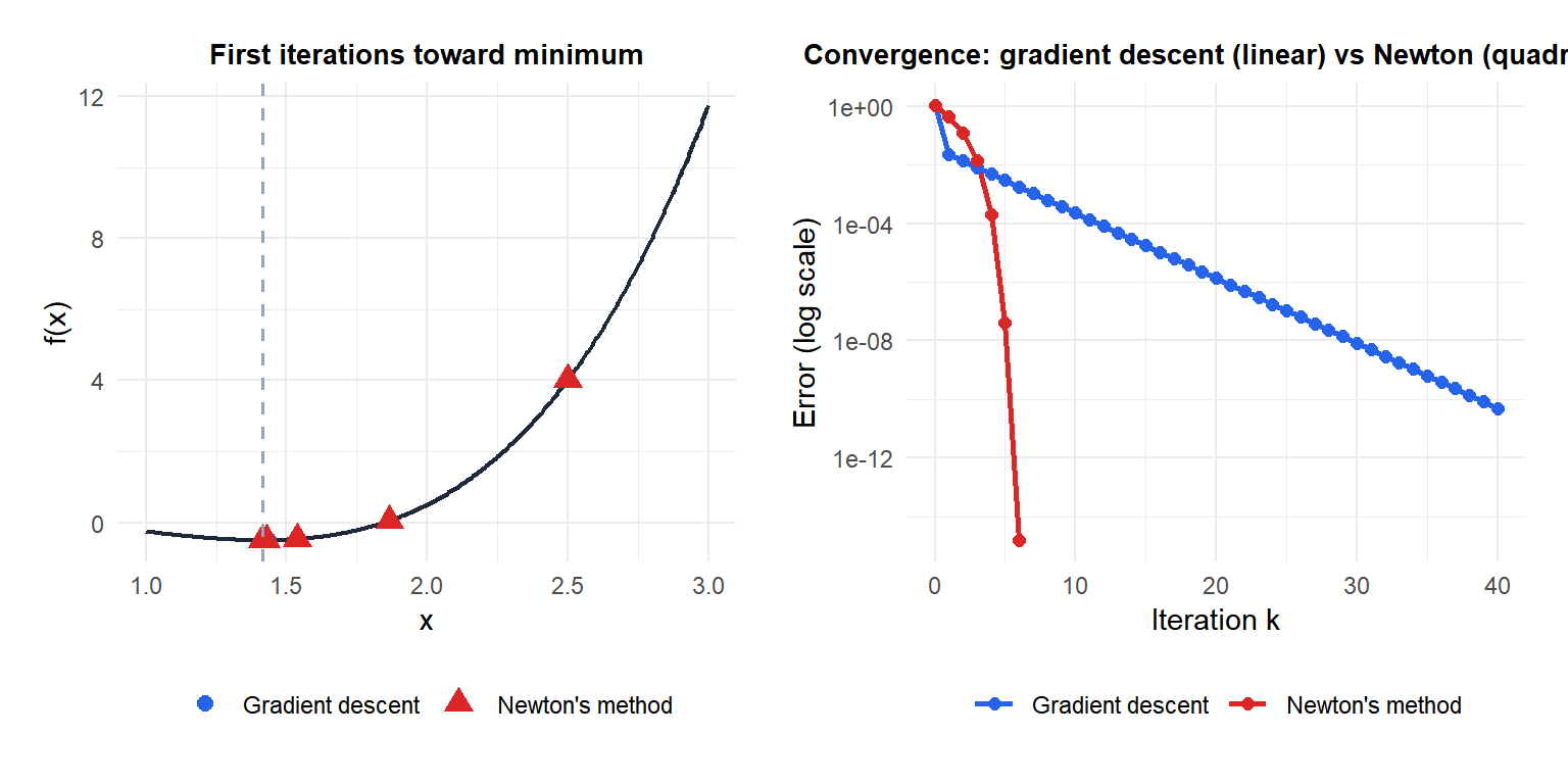
Newton’s method (red) reaches machine precision in 6 iterations. Gradient descent (blue) still has noticeable error after 40 iterations.
Limitations of Newton’s method
Despite quadratic convergence, Newton’s method has three serious practical limitations:
Cost per iteration: computing \(H_k\) requires \(O(n^2)\) entries; solving \(H_k p_k = -g_k\) requires \(O(n^3)\) operations (LU or Cholesky factorization). For \(n = 10^4\) parameters (a small neural network), this is \(10^{12}\) operations per step: completely impractical.
Hessian indefiniteness: far from the optimum, \(H_k\) may not be positive definite. The Newton step \(p_k = -H_k^{-1}g_k\) may then point uphill. Modified Newton methods add a regularization term: \(p_k = -(H_k + \lambda_k I)^{-1}g_k\) with \(\lambda_k\) chosen to ensure positive definiteness (Levenberg-Marquardt strategy).
Convergence is only local: quadratic convergence is guaranteed only near \(x^*\). Starting far away, Newton’s method can diverge or cycle. Always combine with a line search or trust region to ensure global convergence.
⚠️ Newton steps can diverge without safeguards
A pure Newton step without a line search can overshoot the minimum and diverge, especially when the Hessian is nearly singular or indefinite. In practice, Newton’s method is always implemented with either a backtracking line search (reduce step size until sufficient decrease is achieved) or a trust region (restrict the step norm to a ball where the quadratic approximation is reliable).
Quasi-Newton methods
Quasi-Newton methods approximate the Hessian (or its inverse) from gradient differences, avoiding explicit second-derivative computation. They achieve superlinear convergence: slower than Newton’s quadratic, but much faster than gradient descent’s linear convergence.
The key idea: use the change in gradient between successive iterates to update the Hessian approximation. If \(s_k = x_{k+1} - x_k\) and \(y_k = g_{k+1} - g_k\), the updated Hessian approximation \(B_{k+1}\) must satisfy the secant condition:
\[B_{k+1} s_k = y_k\]
This ensures the approximation is consistent with the observed curvature in the direction of the last step.
BFGS update
The Broyden-Fletcher-Goldfarb-Shanno (BFGS) update is the most successful quasi-Newton method. It updates the inverse Hessian approximation \(H_k^{-1} \approx B_k^{-1}\) directly:
\[B_{k+1}^{-1} = \left(I - \rho_k s_k y_k^T\right) B_k^{-1} \left(I - \rho_k y_k s_k^T\right) + \rho_k s_k s_k^T\]
\[\rho_k = \frac{1}{y_k^T s_k}\]
The BFGS update is a rank-2 update of the inverse Hessian: it adds information from the current step and gradient change. Key properties:
- Preserves symmetry: \(B_{k+1}^{-1}\) is symmetric if \(B_k^{-1}\) is.
- Preserves positive definiteness (when \(y_k^T s_k > 0\), guaranteed by a Wolfe line search).
- Requires only \(O(n^2)\) storage and \(O(n^2)\) operations per update.
- Converges superlinearly: \(\|x_{k+1} - x^*\| = o(\|x_k - x^*\|)\), meaning the convergence rate itself improves at each step.
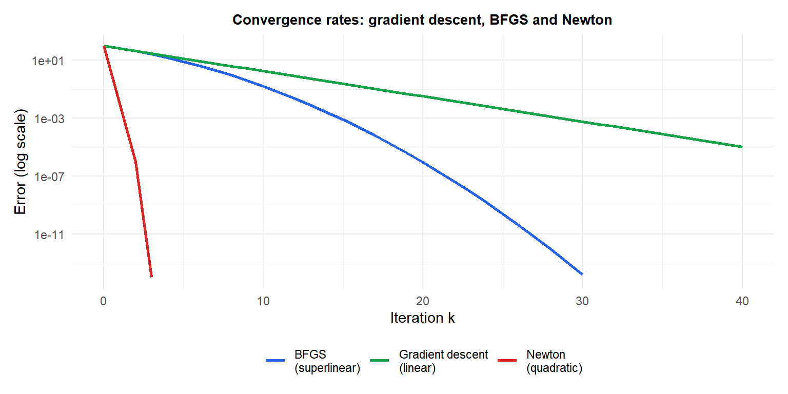
BFGS (blue) sits between gradient descent (green, slow linear) and Newton (red, quadratic): it converges much faster than gradient descent without the \(O(n^3)\) cost of Newton.
L-BFGS: large-scale quasi-Newton
BFGS stores the full \(n \times n\) inverse Hessian approximation, requiring \(O(n^2)\) memory. For \(n = 10^6\) parameters (a typical deep learning model), this is completely infeasible.
Limited-memory BFGS (L-BFGS) stores only the last \(m\) curvature pairs \(\{(s_k, y_k)\}_{k=t-m}^{t-1}\) (typically \(m = 5\) to 20) and implicitly represents the Hessian approximation through these pairs. The matrix-vector product \(B_k^{-1} g_k\) is computed via a two-loop recursion in \(O(mn)\) time and \(O(mn)\) memory.
L-BFGS is the standard algorithm for large-scale smooth unconstrained optimization. It is used in logistic regression, Gaussian process fitting, and many machine learning applications where the Hessian is too large to store.
| Method | Convergence | Cost/iteration | Memory | Best for |
|---|---|---|---|---|
| Gradient descent | Linear | \(O(n)\) | \(O(n)\) | Very large \(n\), non-smooth |
| BFGS | Superlinear | \(O(n^2)\) | \(O(n^2)\) | Medium \(n\) (\(\leq 10^4\)) |
| L-BFGS | Superlinear | \(O(mn)\) | \(O(mn)\) | Large \(n\) (\(> 10^4\)) |
| Newton | Quadratic | \(O(n^3)\) | \(O(n^2)\) | Small \(n\) (\(\leq 10^3\)), exact Hessian available |
Line search and the Wolfe conditions
All quasi-Newton methods require a line search at each step to choose the step size \(\alpha_k\). The Wolfe conditions are standard:
Sufficient decrease (Armijo): \(f(x_k + \alpha_k p_k) \leq f(x_k) + c_1 \alpha_k g_k^T p_k\)
Curvature condition: \(g(x_k + \alpha_k p_k)^T p_k \geq c_2 g_k^T p_k\)
with \(0 < c_1 < c_2 < 1\) (typically \(c_1 = 10^{-4}\), \(c_2 = 0.9\)). The curvature condition ensures \(y_k^T s_k > 0\), which is required for BFGS to maintain positive definiteness of the Hessian approximation.
💡 Newton and BFGS in R
# optim() implements BFGS and L-BFGS-B
f      <- function(x) x[1]^4/4 - x[1]^2 + x[2]^2
grad_f <- function(x) c(x[1]^3 - 2*x[1], 2*x[2])

# BFGS
optim(c(2, 1), f, grad_f, method="BFGS")

# L-BFGS-B (with box constraints)
optim(c(2, 1), f, grad_f, method="L-BFGS-B",
      lower=c(-Inf,-Inf), upper=c(Inf,Inf))

# Newton's method via nlm()
nlm(f, c(2, 1), hessian=TRUE)

# For constrained problems: nloptr with BFGS
library(nloptr)
nloptr(x0=c(2,1), eval_f=f, eval_grad_f=grad_f,
       opts=list(algorithm="NLOPT_LD_LBFGS"))
In practice, always provide the gradient analytically when available: numerical differentiation is slower and less accurate.

