Introduction to optimization
Mathematical optimization finds the values of decision variables that minimize or maximize an objective function, possibly subject to constraints. It is the foundation of machine learning, operations research, economics, and engineering design.
The optimization problem
The general form of an optimization problem is:
\[\min_{x \in \mathcal{X}} f(x) \quad \text{subject to} \quad g_i(x) \leq 0,\; i=1,\ldots,m \quad h_j(x) = 0,\; j=1,\ldots,p\]
where:
- \(x \in \mathbb{R}^n\): decision variables (what we control).
- \(f: \mathbb{R}^n \to \mathbb{R}\): objective function (what we optimize).
- \(g_i(x) \leq 0\): inequality constraints (feasibility region boundary).
- \(h_j(x) = 0\): equality constraints (must be satisfied exactly).
- \(\mathcal{X}\): feasible set (all \(x\) satisfying the constraints).
A maximization problem \(\max f(x)\) is equivalent to \(\min -f(x)\).
Examples across domains:
- Machine learning: minimize the loss function \(f(\theta) = \frac{1}{n}\sum_i \ell(y_i, \hat{y}_i(\theta))\) over model parameters \(\theta\).
- Portfolio optimization: maximize expected return subject to a variance constraint.
- Route planning: minimize travel time subject to road network constraints.
- Production planning: maximize profit subject to resource capacity constraints.
Taxonomy of optimization problems
Continuous vs discrete
- Continuous: \(x \in \mathbb{R}^n\). Gradient-based methods apply. Examples: neural network training, regression.
- Discrete (combinatorial): \(x \in \mathbb{Z}^n\) or \(x \in \{0,1\}^n\). Much harder in general. Examples: scheduling, routing, integer programming.
- Mixed-integer: some variables continuous, some discrete.
Constrained vs unconstrained
- Unconstrained: \(\mathcal{X} = \mathbb{R}^n\). Optimality characterized purely by derivatives.
- Constrained: the feasible set is a proper subset of \(\mathbb{R}^n\). Requires Lagrange multipliers or KKT conditions.
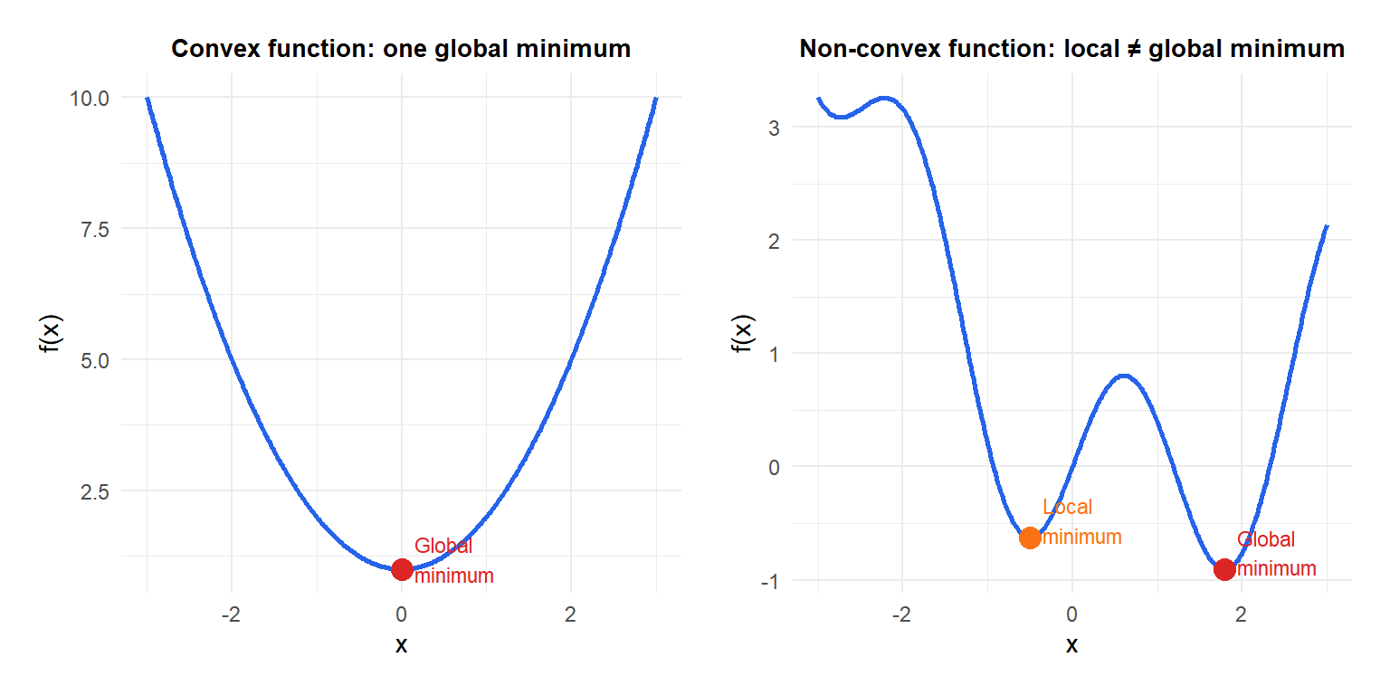
Convex vs non-convex
The most important distinction in practice:
- Convex: \(f\) is convex and \(\mathcal{X}\) is a convex set. Every local minimum is a global minimum. Efficient algorithms exist with convergence guarantees.
- Non-convex: multiple local minima possible. No guarantee that any algorithm finds the global minimum. Most deep learning problems are non-convex.
Optimality conditions
First-order necessary condition (unconstrained)
If \(x^*\) is a local minimum of a differentiable \(f\), then:
\[\nabla f(x^*) = \mathbf{0}\]
Points where \(\nabla f = 0\) are called stationary points or critical points. They include minima, maxima, and saddle points.
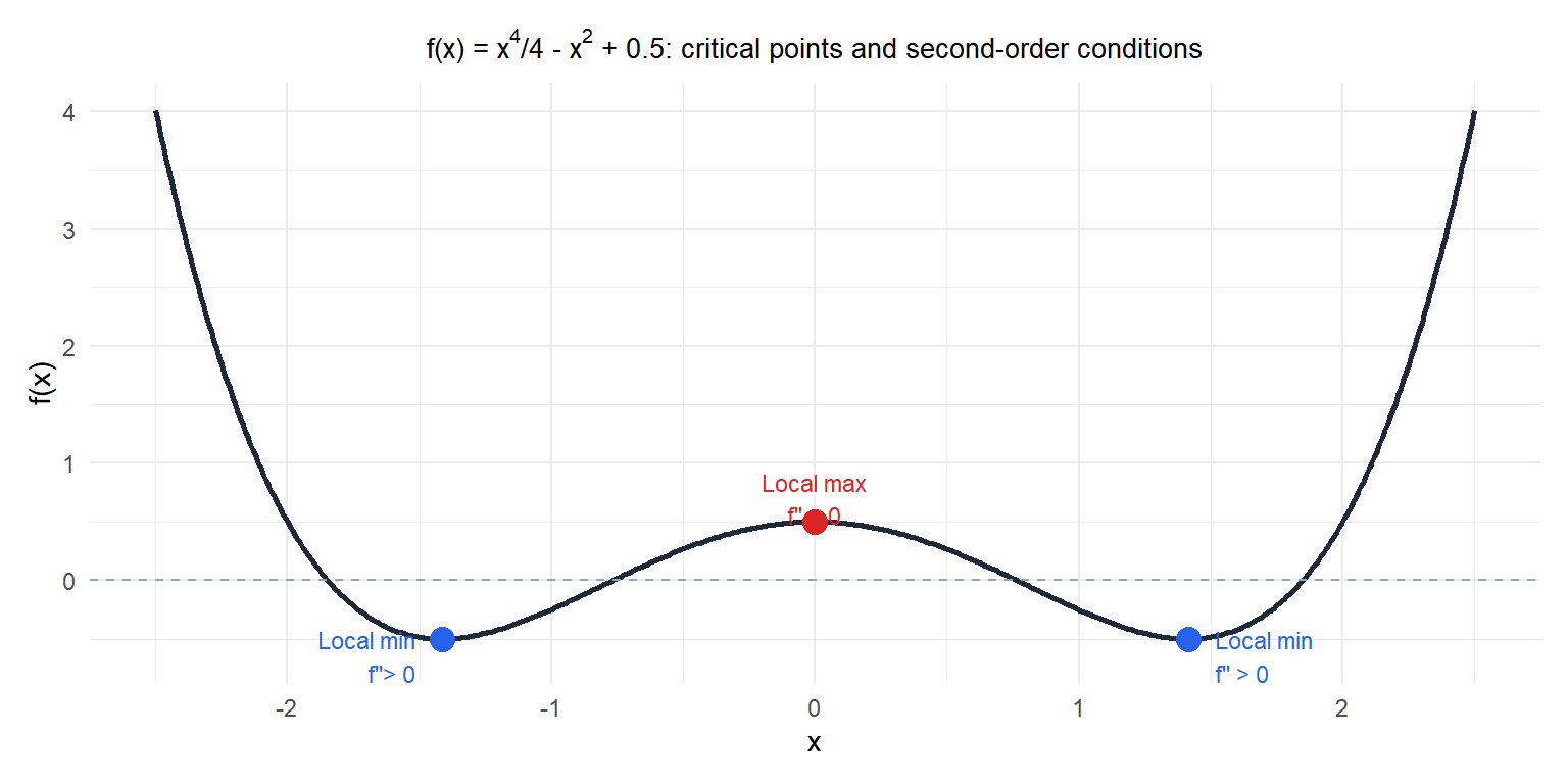
Second-order conditions (unconstrained)
At a stationary point \(x^*\):
| Hessian \(\nabla^2 f(x^*)\) | Type of critical point |
|---|---|
| Positive definite | Local minimum |
| Negative definite | Local maximum |
| Indefinite | Saddle point |
| Positive semidefinite | Cannot determine (need higher-order analysis) |
For a function of one variable: \(f''(x^*) > 0\) implies local minimum; \(f''(x^*) < 0\) implies local maximum.
Constrained optimality: Lagrange and KKT
For constrained problems, the gradient of \(f\) at the optimum is not necessarily zero. Instead, it must be expressible as a linear combination of the constraint gradients.
For equality-constrained problems (\(h_j(x) = 0\) only), the Lagrange conditions require:
\[\nabla f(x^*) + \sum_j \lambda_j \nabla h_j(x^*) = \mathbf{0}\]
For problems with both equality and inequality constraints, the KKT (Karush-Kuhn-Tucker) conditions generalize this, adding complementary slackness conditions for the inequality constraints. These are covered in detail in the Lagrange multipliers and KKT posts.
Overview of solution methods
| Method | Problem type | Key idea |
|---|---|---|
| Simplex | Linear programming | Move along vertices of feasible polytope |
| Gradient descent | Unconstrained, differentiable | Follow negative gradient |
| Newton’s method | Unconstrained, twice differentiable | Use Hessian to take curved steps |
| BFGS / L-BFGS | Unconstrained, large-scale | Approximate Hessian efficiently |
| Lagrange multipliers | Equality-constrained | Augment objective with constraint penalties |
| Interior point | Convex, constrained | Stay inside feasible region |
| Dijkstra | Shortest path on graphs | Greedy expansion of nearest node |
| Simulated annealing | Non-convex, combinatorial | Accept worse solutions probabilistically |
⚠️ Local methods can get stuck in local minima
Gradient-based methods (gradient descent, Newton’s method, BFGS) converge to a local minimum, not necessarily the global one. For non-convex problems this is a fundamental limitation:
- Convex problems: any local minimum is global. Use gradient-based methods with confidence.
- Non-convex problems (neural networks, combinatorial optimization): local methods may find poor solutions. Strategies include multiple random restarts, stochastic methods, or global optimization heuristics (simulated annealing, genetic algorithms).
In practice, many non-convex problems in machine learning have good empirical behavior: saddle points dominate over local minima, and most local minima have similar objective values.
💡 Choosing the right optimization method
Key questions before selecting a method:
- Is the problem convex? If yes, any local solver finds the global optimum.
- Is \(f\) differentiable? Gradient-based methods require at least first derivatives.
- How many variables? Large-scale problems (\(n > 10^4\)) need methods that avoid storing the Hessian (L-BFGS, SGD).
- Are there constraints? Equality only → Lagrange. Inequality too → KKT, interior point, or penalty methods.
- Is the problem combinatorial? Use integer programming, dynamic programming, or metaheuristics.

