Introduction to graphs
A graph is a mathematical structure that models pairwise relationships between objects. Road networks, social connections, dependency trees, electrical circuits, and the internet are all graphs. Graph algorithms solve fundamental problems on these structures: finding shortest paths, detecting cycles, spanning networks with minimum cost, and clustering connected components.
Definition
A graph \(G = (V, E)\) consists of:
- \(V\): a set of vertices (also called nodes). \(|V| = n\).
- \(E\): a set of edges (also called arcs or links), each connecting a pair of vertices. \(|E| = m\).
An edge between vertices \(u\) and \(v\) is written \((u,v)\) or \(\{u,v\}\).
The degree of a vertex \(v\), written \(\deg(v)\), is the number of edges incident to \(v\). For directed graphs: in-degree (edges arriving) and out-degree (edges leaving).
Handshaking lemma: \(\sum_{v \in V} \deg(v) = 2m\) (each edge contributes 2 to the total degree sum).
Types of graphs
Directed vs undirected
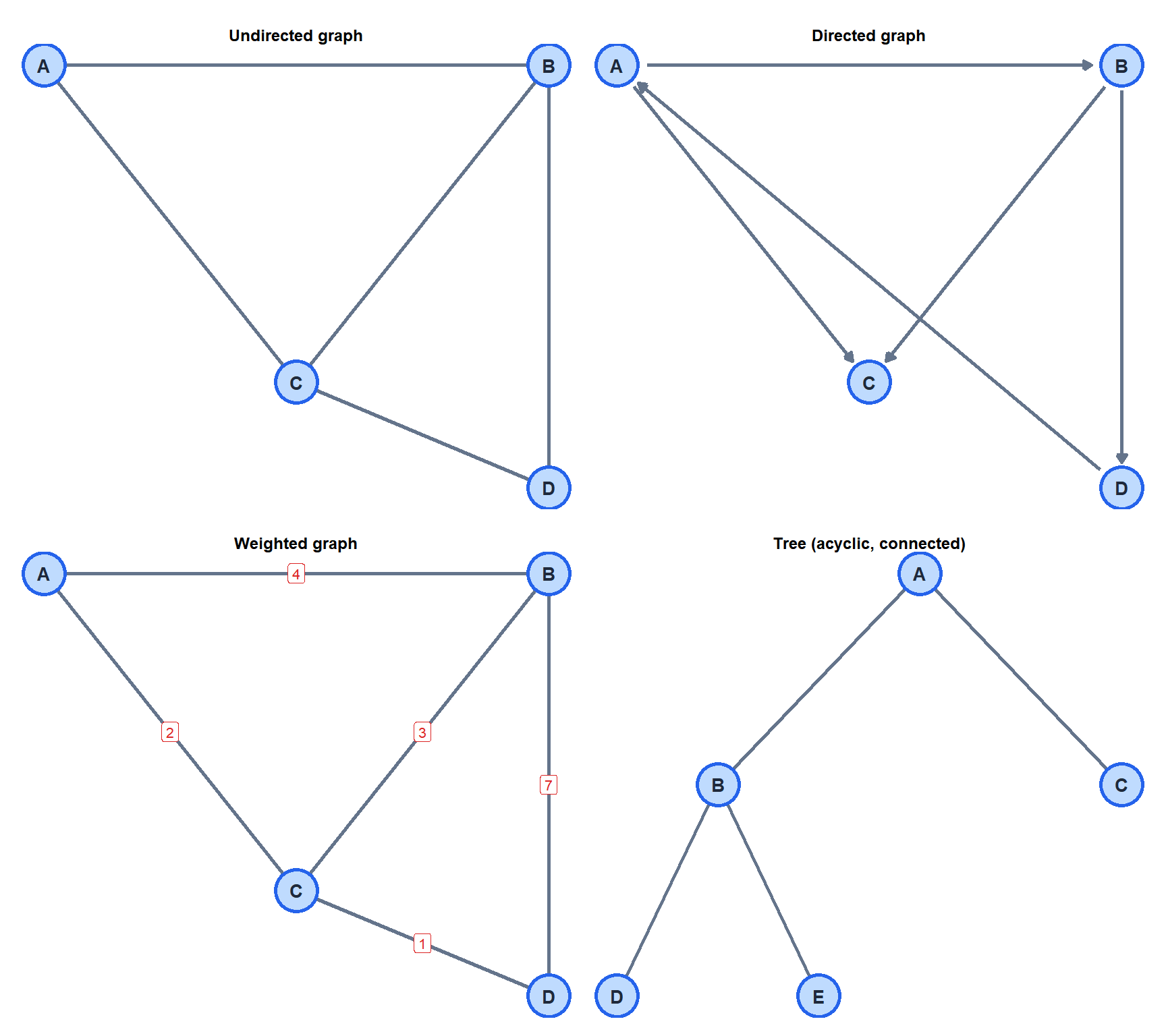
In an undirected graph, edges have no direction: \((u,v)\) and \((v,u)\) are the same edge. Road networks where streets go both ways, friendship networks.
In a directed graph (digraph), each edge has a direction: \((u,v)\) goes from \(u\) to \(v\) but not necessarily from \(v\) to \(u\). Web links, citation networks, dependency graphs.
Weighted vs unweighted
In a weighted graph, each edge carries a numerical weight \(w(u,v)\): distance, cost, capacity, time. Unweighted graphs treat all edges equally (or equivalently, all weights are 1).
Connected vs disconnected
An undirected graph is connected if there is a path between every pair of vertices. A connected component is a maximal connected subgraph. A directed graph is strongly connected if every vertex is reachable from every other vertex.
Cyclic vs acyclic
A cycle is a path that starts and ends at the same vertex. A graph with no cycles is acyclic. A connected acyclic undirected graph is a tree: it has exactly \(n-1\) edges and a unique path between any two vertices.
Graph representations
Two standard data structures for storing graphs in memory:
Adjacency matrix
An \(n \times n\) matrix \(A\) where \(A_{ij} = 1\) (or \(w_{ij}\) for weighted graphs) if there is an edge from \(i\) to \(j\), and 0 otherwise.
For the undirected graph above (A, B, C, D):
\[A = \begin{pmatrix} 0 & 1 & 1 & 0 \\ 1 & 0 & 1 & 1 \\ 1 & 1 & 0 & 1 \\ 0 & 1 & 1 & 0 \end{pmatrix}\]
Advantages: \(O(1)\) edge lookup; natural for dense graphs. Disadvantages: \(O(n^2)\) memory regardless of the number of edges; inefficient for sparse graphs.
Adjacency list
Each vertex stores a list of its neighbors. For the same graph:
A: [B, C]
B: [A, C, D]
C: [A, B, D]
D: [B, C]Advantages: \(O(n + m)\) memory; efficient for sparse graphs (most real networks). Disadvantages: \(O(\deg(v))\) edge lookup.
| Adjacency matrix | Adjacency list | |
|---|---|---|
| Memory | \(O(n^2)\) | \(O(n + m)\) |
| Edge lookup \((u,v)\) | \(O(1)\) | \(O(\deg(u))\) |
| Iterate over neighbors of \(v\) | \(O(n)\) | \(O(\deg(v))\) |
| Best for | Dense graphs (\(m \approx n^2\)) | Sparse graphs (\(m \ll n^2\)) |
Most real-world graphs (road networks, social networks, web graphs) are sparse: \(m = O(n)\) or \(O(n \log n)\). Adjacency lists are almost always the right choice.
Paths, cycles and connectivity
A path from \(u\) to \(v\) is a sequence of vertices \(u = v_0, v_1, \ldots, v_k = v\) where each consecutive pair \((v_i, v_{i+1})\) is an edge. The length of the path is the number of edges (\(k\)) for unweighted graphs, or the sum of edge weights for weighted graphs.
A simple path visits each vertex at most once. A cycle is a path where \(v_0 = v_k\) and at least one edge is traversed. A simple cycle visits each vertex exactly once (except the start/end).
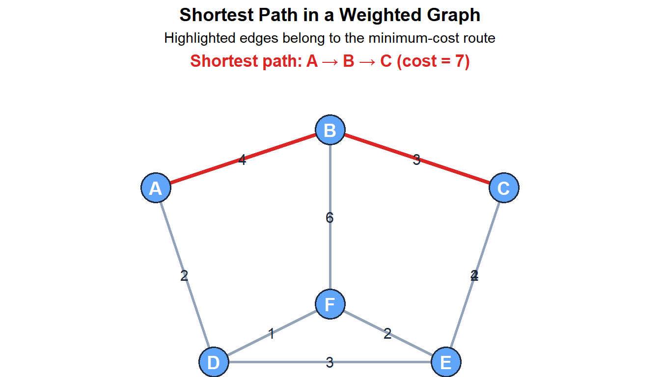
The shortest path from \(u\) to \(v\) is the path with minimum total weight. Finding shortest paths is one of the most important problems in graph theory and the subject of Dijkstra’s algorithm.
Special graph families
Several graph families appear frequently in algorithms and applications:
- Tree: connected acyclic undirected graph. \(n\) vertices, \(n-1\) edges. Unique path between any two vertices.
- Forest: acyclic undirected graph (union of trees). No unique path requirement.
- DAG (Directed Acyclic Graph): directed graph with no directed cycles. Used for dependency resolution, topological sorting, dynamic programming.
- Bipartite graph: vertices split into two sets \(U\) and \(V\); all edges go between \(U\) and \(V\). Models matchings (jobs to workers, students to courses).
- Complete graph \(K_n\): every pair of vertices is connected. \(m = n(n-1)/2\) edges.
- Planar graph: can be drawn in the plane without edge crossings. Road networks are often nearly planar.
💡 Graphs in R
library(igraph)

# Create an undirected weighted graph
g <- graph_from_edgelist(
  matrix(c("A","B", "A","C", "B","C", "B","D", "C","D"),
         ncol=2, byrow=TRUE),
  directed=FALSE
)
E(g)$weight <- c(4, 2, 3, 7, 1)

# Basic properties
vcount(g)       # number of vertices
ecount(g)       # number of edges
degree(g)       # degree of each vertex
is_connected(g) # TRUE/FALSE

# Adjacency matrix
as_adjacency_matrix(g, attr="weight")

# Shortest path (uses Dijkstra internally)
shortest_paths(g, from="A", to="D", weights=E(g)$weight)
distances(g, weights=E(g)$weight)  # full distance matrix

# Plot
plot(g, edge.label=E(g)$weight, vertex.color="#bfdbfe",
     edge.color="#64748b", vertex.label.color="#1e293b")
