Integer programming
Integer programming (IP) optimizes a linear objective over variables constrained to take integer or binary values. The integrality requirement shatters the convexity that makes LP tractable: the feasible set is a discrete collection of points, and the LP simplex method no longer applies directly. Most practical combinatorial problems, including scheduling, routing, resource allocation, are integer programs.
Formulation
A Mixed Integer Linear Program (MILP) has the form:
\[\min_{x,y} \mathbf{c}^T x + \mathbf{d}^T y \quad \text{s.t.} \quad \mathbf{A}x + \mathbf{B}y \leq \mathbf{b}, \quad x \geq 0, \quad y \in \mathbb{Z}^p\]
where \(x\) are continuous variables and \(y\) are integer variables. When all variables are integer: Integer Linear Program (ILP). When all variables are binary (\(y \in \{0,1\}^p\)): Binary Integer Program (BIP).
Binary variables are particularly expressive: they model yes/no decisions, logical conditions, and combinatorial structures. Almost any combinatorial optimization problem can be formulated as a BIP.
Knapsack: \(n\) items with values \(v_i\) and weights \(w_i\). Maximize total value subject to weight capacity \(W\):
\[\max \sum_i v_i x_i \quad \text{s.t.} \quad \sum_i w_i x_i \leq W, \quad x_i \in \{0,1\}\]
Assignment: assign \(n\) workers to \(n\) jobs (one-to-one). Minimize total cost \(c_{ij}\):
\[\min \sum_{i,j} c_{ij} x_{ij} \quad \text{s.t.} \quad \sum_j x_{ij} = 1 \;\forall i, \quad \sum_i x_{ij} = 1 \;\forall j, \quad x_{ij} \in \{0,1\}\]
Fixed-charge facility location: decide which facilities to open (\(y_j \in \{0,1\}\)) and how much to ship from each (\(x_{ij} \geq 0\)):
\[\min \sum_j f_j y_j + \sum_{i,j} c_{ij} x_{ij} \quad \text{s.t.} \quad \sum_j x_{ij} \geq d_i \;\forall i, \quad x_{ij} \leq M y_j \;\forall i,j\]
Why integrality makes optimization hard
Adding integrality constraints to an LP changes the problem fundamentally. The LP feasible region is a convex polytope; the IP feasible region is the discrete set of integer points inside that polytope. Two key consequences:
No gradient to follow: the objective is linear and the feasible set is discrete. Gradient-based methods do not apply. Rounding the LP solution to the nearest integer point often gives an infeasible or highly suboptimal solution.
NP-hardness: integer programming is NP-hard in general. The knapsack problem, traveling salesman, bin packing, and scheduling are all NP-hard IP problems. No polynomial-time algorithm is known (and none is expected to exist under \(P \neq NP\)).
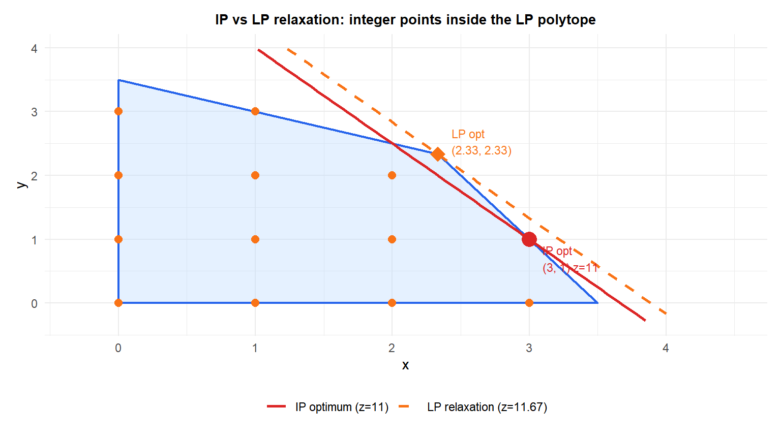
The LP relaxation optimum (orange diamond) is non-integer at \((2.33, 2.33)\) with \(z=11.67\). The true IP optimum (red dot) is at \((3,1)\) with \(z=11\). The LP optimum provides an upper bound on the IP objective (for maximization).
The LP relaxation and bounds
The LP relaxation drops the integrality constraints and solves the resulting LP. For a maximization problem:
\[z_\text{LP} \geq z_\text{IP}\]
The LP relaxation gives an upper bound on the IP objective (lower bound for minimization). The gap \(z_\text{LP} - z_\text{IP}\) measures how much the integrality constraints cost.
If the LP relaxation solution happens to be integer-valued, it is also the IP optimum. For special problem structures (totally unimodular constraint matrices, e.g., network flow problems, assignment problems), the LP relaxation always gives an integer solution: no branch and bound is needed.
Branch and bound
Branch and bound is the fundamental algorithm for solving integer programs. It implicitly enumerates all integer feasible solutions by partitioning the problem into subproblems and using LP relaxations to prune subproblems that cannot contain the optimal solution.
Algorithm:
Initialize: solve the LP relaxation. If the solution is integer, done. Otherwise, the LP optimal value is an upper bound \(\bar{z}\) (for maximization). Set the best integer solution found so far \(\underline{z} = -\infty\).
Branch: select a fractional variable \(x_j = \bar{x}_j\) (non-integer). Create two child subproblems by adding:
- Branch down: \(x_j \leq \lfloor \bar{x}_j \rfloor\)
- Branch up: \(x_j \geq \lceil \bar{x}_j \rceil\)
Bound: solve the LP relaxation of each child. If the LP optimum is:
- Infeasible: prune (no feasible integer solution in this branch).
- Worse than \(\underline{z}\): prune (cannot improve the best known solution).
- Integer: update \(\underline{z}\) if better than current best.
- Fractional and better than \(\underline{z}\): add to the list of open nodes.
Repeat until no open nodes remain. The best integer solution found is optimal.
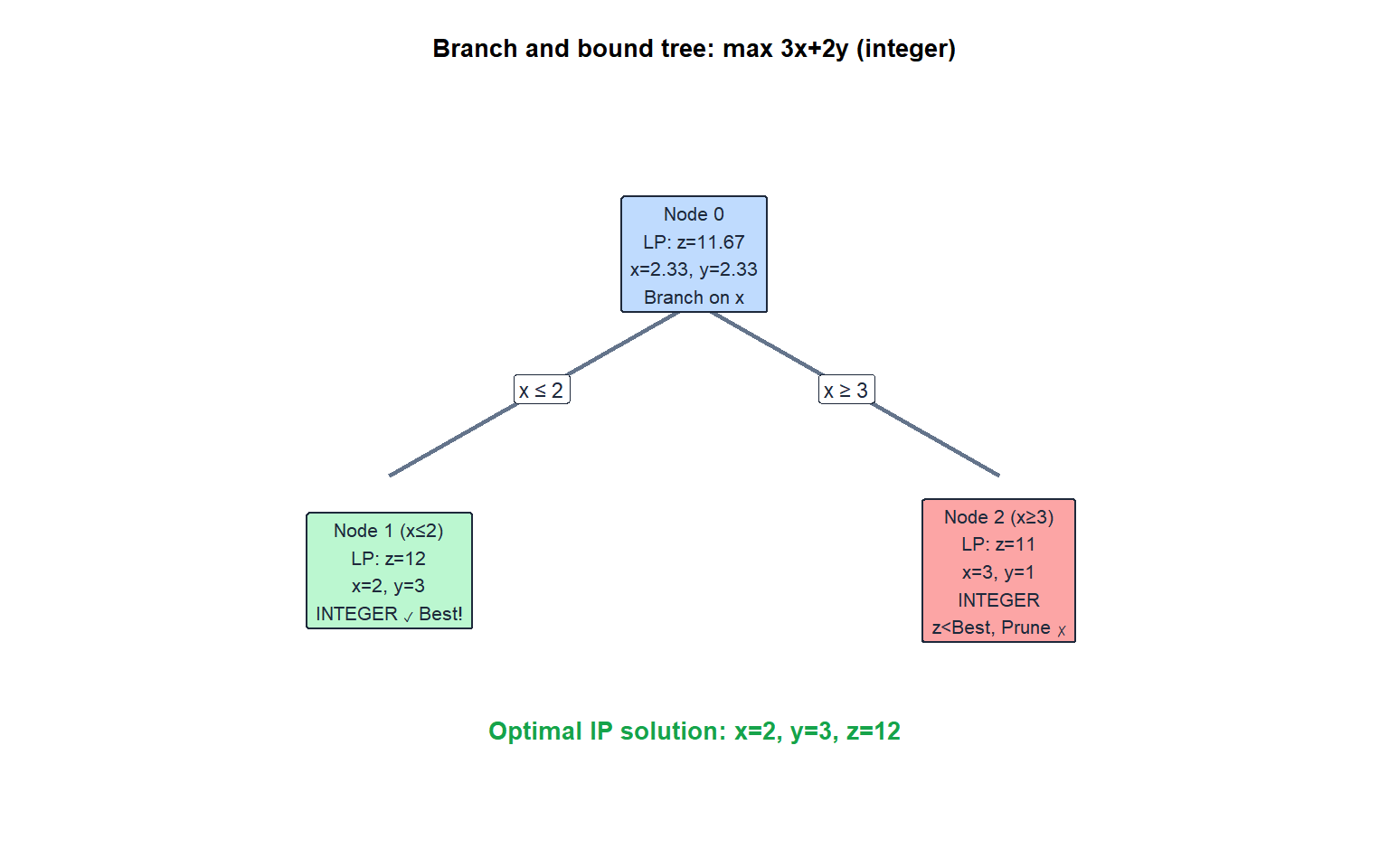
The algorithm finds the optimal solution \((x=2, y=3, z=12)\) by solving only 3 LP relaxations instead of enumerating all integer points.
Cutting planes
Cutting planes are additional linear inequalities added to the LP relaxation to cut off fractional solutions without removing any integer feasible points. They tighten the LP relaxation, bringing its optimum closer to the IP optimum.
The most important cutting planes:
Gomory cuts: derived algebraically from the LP tableau. For a fractional basic variable \(x_j = \bar{x}_j\) with \(\bar{x}_j \notin \mathbb{Z}\), the Gomory cut removes the fractional LP solution while keeping all integer solutions feasible.
Cover inequalities (for knapsack): if a subset \(S\) of items cannot all fit in the knapsack (\(\sum_{i \in S} w_i > W\)), then at most \(|S|-1\) of them can be selected: \(\sum_{i \in S} x_i \leq |S|-1\).
Modern IP solvers (Gurobi, CPLEX) combine branch and bound with cutting planes (branch and cut): cuts are generated at each node of the branch and bound tree to tighten the local LP relaxation.
⚠️ Integer programming is NP-hard: beware of problem size
Even with modern solvers, integer programs can be intractable for large instances:
- A binary IP with \(n=50\) variables has \(2^{50} \approx 10^{15}\) feasible points in the worst case.
- The Traveling Salesman Problem with \(n\) cities has \((n-1)!/2\) possible tours.
- Practical solvability depends heavily on problem structure. Network flow IPs (totally unimodular) solve like LPs. General IPs with poor LP relaxation bounds can take hours or fail to solve.
Before formulating a problem as an IP, check: is the LP relaxation tight? Does the constraint matrix have special structure (total unimodularity)? Is a heuristic or approximation algorithm acceptable?
Applications
Integer programming models an enormous range of real problems:
- Airline scheduling: assigning aircraft and crews to flights, respecting rest requirements and hub connections.
- Supply chain: warehouse location, inventory routing, vehicle scheduling.
- Telecommunications: network design, frequency assignment.
- Finance: portfolio selection with transaction costs, cardinality constraints.
- Healthcare: nurse scheduling, operating room planning, vaccine distribution.
💡 Integer programming in R
library(lpSolve)

# Knapsack: 5 items, values and weights
values  <- c(10, 6, 3, 7, 8)
weights <- c(5,  3, 2, 4, 5)
capacity <- 10

obj <- values
mat <- matrix(weights, nrow=1)
rhs <- capacity
dir <- "<="

# Binary IP (all.bin=TRUE)
sol <- lp("max", obj, mat, dir, rhs, all.bin=TRUE)
sol$solution  # which items to take
sol$objval    # optimal value

# Mixed integer with lpSolve
# int.vec specifies which variables must be integer
sol <- lp("max", obj, mat, dir, rhs, int.vec=1:5)

# For serious MIP solving: use highs package (faster)
library(highs)
highs_solve(L=obj, lower=rep(0,5), upper=rep(1,5),
            A=matrix(weights,1), lhs=-Inf, rhs=capacity,
            types=rep("I",5), maximum=TRUE)
For production-grade IP solving in R, highs provides the HiGHS solver (state-of-the-art open-source MIP solver). Commercial options (Gurobi, CPLEX) are significantly faster for large instances.

