Gradient descent
Gradient descent minimizes a differentiable function \(f(x)\) by repeatedly moving in the direction opposite to the gradient, which is the direction of steepest ascent. It is the foundational algorithm behind training neural networks, logistic regression, and virtually every large-scale machine learning model.
Intuition
Imagine standing on a hilly landscape in thick fog. You cannot see the valley, but you can feel the slope under your feet. The steepest descent strategy: at each step, move in the direction where the ground drops most steeply. Repeat until you reach a flat point.
The gradient \(\nabla f(x)\) points in the direction of steepest ascent. Moving opposite to it, \(-\nabla f(x)\), gives the direction of steepest descent. The step size (how far to move) is controlled by the learning rate \(\alpha > 0\).
The update rule
\[x_{k+1} = x_k - \alpha \nabla f(x_k)\]
Starting from an initial point \(x_0\), this is applied iteratively until a stopping criterion is met: \(\|\nabla f(x_k)\| < \varepsilon\), maximum iterations reached, or the improvement in \(f\) falls below a threshold.
For a function of one variable: \(x_{k+1} = x_k - \alpha f'(x_k)\). The update subtracts the slope scaled by \(\alpha\).
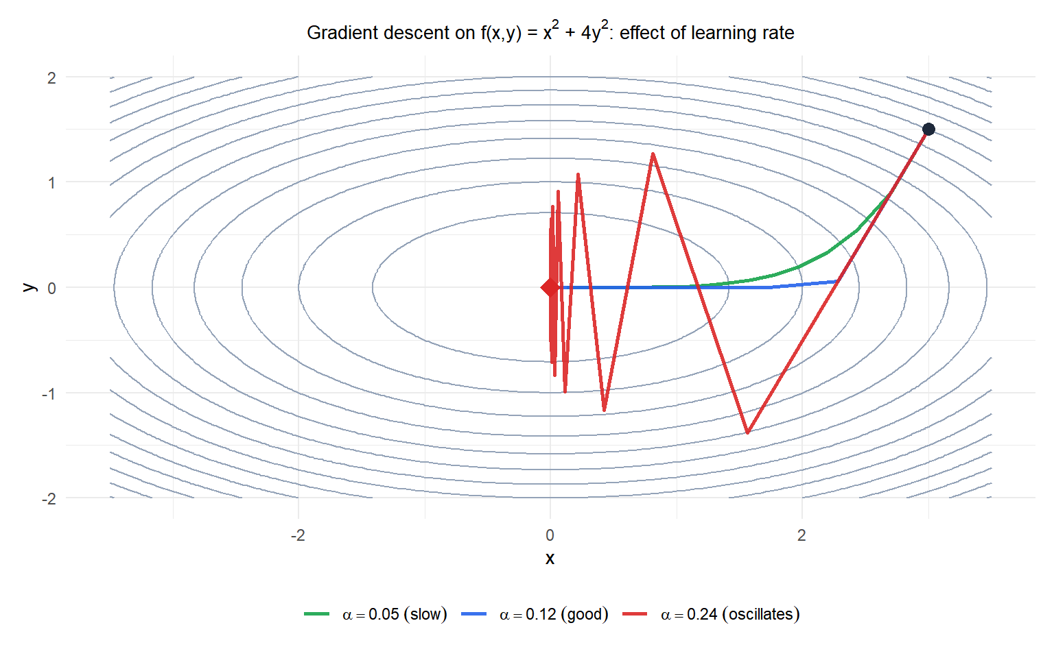
Low learning rate (green) converges safely but slowly. Good learning rate (blue) converges in few iterations. High learning rate (red) oscillates across the valley: the elliptical shape means the \(y\)-direction has much steeper curvature, and large steps overshoot.
The learning rate
The learning rate \(\alpha\) is the most important hyperparameter in gradient descent. For a function with Lipschitz-continuous gradient (gradient does not change too fast), the optimal fixed learning rate satisfies:
\[\alpha \leq \frac{1}{L}\]
where \(L\) is the Lipschitz constant of the gradient: \(\|\nabla f(x) - \nabla f(y)\| \leq L\|x-y\|\) for all \(x, y\). For the quadratic \(f(x) = \frac{1}{2}x^T H x\), \(L\) equals the largest eigenvalue of \(H\).
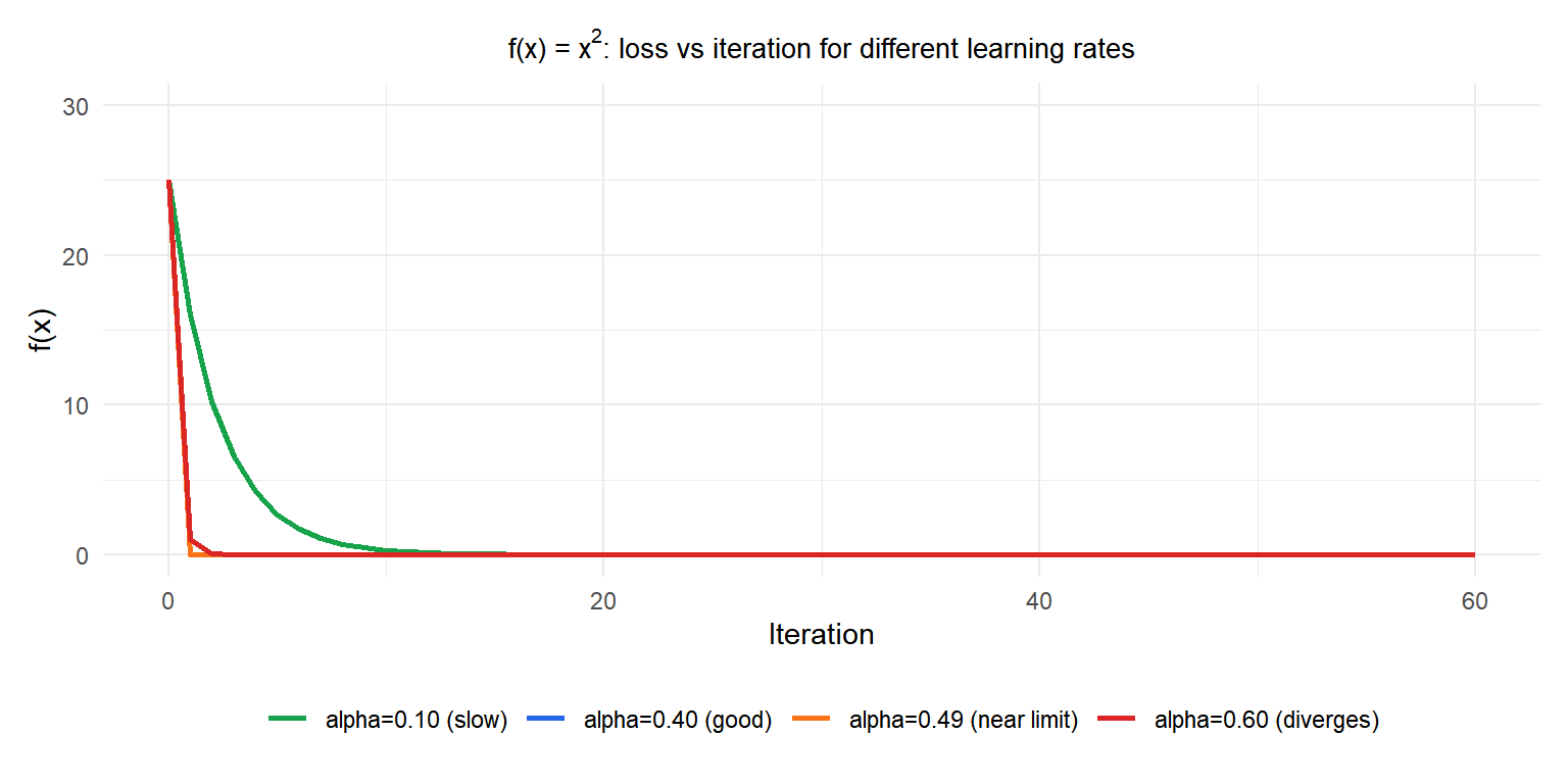
For \(f(x)=x^2\), the Lipschitz constant is \(L=2\) and the safe threshold is \(\alpha \leq 0.5\). At \(\alpha=0.49\) (orange) convergence is very slow near the limit; at \(\alpha=0.6\) (red) the iterates diverge.
Convergence theory
For a convex function with \(L\)-Lipschitz gradient, gradient descent with constant step \(\alpha = 1/L\) achieves:
\[f(x_k) - f(x^*) \leq \frac{L \|x_0 - x^*\|^2}{2k}\]
This is sublinear convergence: \(O(1/k)\). To halve the error you need four times as many iterations.
For strongly convex functions (Hessian eigenvalues bounded below by \(\mu > 0\)), convergence is linear (geometric):
\[f(x_k) - f(x^*) \leq \left(1 - \frac{\mu}{L}\right)^k (f(x_0) - f(x^*))\]
The ratio \(\kappa = L/\mu\) is the condition number. Ill-conditioned problems (\(\kappa \gg 1\), elongated contours like the ellipse above) converge very slowly. This is why preconditioning and adaptive methods (Adam, RMSProp) matter.
Batch, stochastic, and mini-batch
In machine learning, \(f(\theta) = \frac{1}{n}\sum_{i=1}^n \ell(\theta; x_i, y_i)\) is a sum over \(n\) training examples. Computing the full gradient requires evaluating all \(n\) terms, which is expensive for large datasets.
Batch gradient descent
Uses the full dataset to compute the gradient at each step. Exact gradient, stable convergence, but slow per iteration for large \(n\).
Stochastic gradient descent (SGD)
Uses a single randomly chosen example \(i\) at each step:
\[x_{k+1} = x_k - \alpha \nabla \ell(\theta; x_{i_k}, y_{i_k})\]
Much faster per iteration. The gradient is a noisy estimate: \(E[\nabla \ell_i] = \nabla f\). This noise prevents exact convergence but helps escape shallow local minima. Requires decreasing learning rate (\(\alpha_k \to 0\)) for theoretical convergence guarantees.
Mini-batch gradient descent
Uses a small batch of \(B\) examples (typically \(B = 32\) to \(512\)):
\[x_{k+1} = x_k - \frac{\alpha}{B} \sum_{i \in \mathcal{B}_k} \nabla \ell(\theta; x_i, y_i)\]
The standard in deep learning. Balances the variance reduction of batching with the speed of SGD. GPU parallelism makes batch computation nearly free for reasonable \(B\).
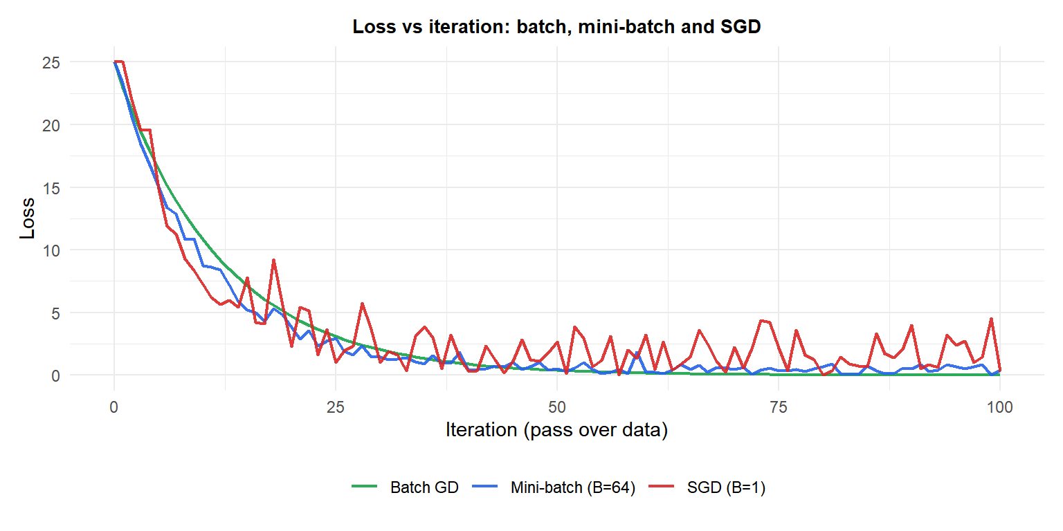
Batch GD (green) descends smoothly but slowly. SGD (red) descends faster initially but oscillates. Mini-batch (blue) balances both: fast descent with moderate noise.
Choosing the learning rate: line search
Instead of a fixed \(\alpha\), line search finds the best step size at each iteration:
\[\alpha_k = \arg\min_{\alpha > 0} f(x_k - \alpha \nabla f(x_k))\]
Exact line search solves this minimization exactly (feasible for simple functions). Backtracking line search is practical: start with a large \(\alpha\) and halve it until the Armijo condition is satisfied:
\[f(x_k - \alpha \nabla f(x_k)) \leq f(x_k) - c \alpha \|\nabla f(x_k)\|^2\]
for some small constant \(c \in (0,1)\) (typically \(c = 10^{-4}\)). This ensures sufficient decrease without requiring exact minimization.
⚠️ Gradient descent fails for non-smooth and non-convex functions
Three situations where vanilla gradient descent is unreliable:
Non-smooth functions: if \(f\) is not differentiable at \(x_k\) (e.g., L1 regularization, ReLU), the gradient does not exist. Use subgradient methods or proximal algorithms instead.
Non-convex functions: gradient descent converges to a stationary point, not necessarily a global minimum. In deep learning this is accepted in practice (most local minima are empirically good), but there is no theoretical guarantee.
Saddle points: in high dimensions, stationary points are usually saddle points (gradient zero but not a minimum). Vanilla gradient descent can get stuck near saddle points for exponentially long. SGD noise and momentum methods (Adam) help escape them faster.
Extensions: momentum and adaptive methods
Vanilla gradient descent is rarely used in deep learning. Two important extensions:
Momentum: accumulates a velocity vector \(v\) in the direction of consistent gradients, dampening oscillations and accelerating convergence in low-curvature directions:
\[v_{k+1} = \beta v_k + \nabla f(x_k), \qquad x_{k+1} = x_k - \alpha v_{k+1}\]
Adam (Adaptive Moment Estimation): maintains per-parameter learning rates based on first and second moment estimates of the gradient. Effectively adapts \(\alpha\) individually for each dimension. The standard optimizer for deep learning.
Nesterov accelerated gradient (NAG): evaluates the gradient at a “lookahead” point \(x_k - \beta v_k\) rather than at \(x_k\), giving better theoretical convergence for convex functions (\(O(1/k^2)\) instead of \(O(1/k)\)).
💡 Gradient descent in R
# Manual gradient descent for any differentiable f
gradient_descent <- function(f, grad_f, x0, alpha=0.01,
                              max_iter=1000, tol=1e-6) {
  x    <- x0
  path <- matrix(NA, max_iter+1, length(x0))
  path[1,] <- x
  for (k in 1:max_iter) {
    g <- grad_f(x)
    x <- x - alpha * g
    path[k+1,] <- x
    if (sqrt(sum(g^2)) < tol) break
  }
  list(x=x, value=f(x), path=path[1:(k+1),])
}

# Example: minimize f(x,y) = x^2 + 4y^2
f     <- function(x) x[1]^2 + 4*x[2]^2
grad_f <- function(x) c(2*x[1], 8*x[2])
result <- gradient_descent(f, grad_f, x0=c(3,1.5), alpha=0.1)

# For machine learning with automatic differentiation: use torch or tensorflow
# For convex optimization: use CVXR which calls interior point solvers
