Dijkstra's algorithm
Dijkstra’s algorithm, developed by Edsger Dijkstra in 1956, finds the shortest path from a source vertex to all other vertices in a weighted graph with non-negative edge weights. It is the foundation of GPS navigation, network routing (OSPF protocol), and map services like Google Maps.
Key idea: greedy expansion
Dijkstra’s algorithm maintains a set of vertices whose shortest distance from the source is already known (the settled set) and a priority queue of candidates ordered by their current best distance estimate. At each step it extracts the closest unsettled vertex, finalizes its distance, and relaxes its outgoing edges.
The correctness relies on non-negative weights: once a vertex is settled, no future path through other vertices can improve its distance. With negative weights this guarantee fails, and Bellman-Ford must be used instead.
The algorithm
Input: a weighted directed graph \(G = (V, E, w)\) with \(w(u,v) \geq 0\), and a source vertex \(s\).
Output: \(d[v]\) = shortest distance from \(s\) to \(v\), and \(\text{prev}[v]\) = predecessor of \(v\) on the shortest path.
Initialization:
\[d[s] = 0, \quad d[v] = \infty \;\forall v \neq s, \quad \text{prev}[v] = \text{None} \;\forall v\]
Insert all vertices into a min-priority queue \(Q\) keyed by \(d[v]\).
Main loop: while \(Q\) is not empty:
- Extract \(u = \arg\min_{v \in Q} d[v]\) (vertex with smallest tentative distance).
- For each neighbor \(v\) of \(u\) with edge weight \(w(u,v)\):
- Relaxation: if \(d[u] + w(u,v) < d[v]\), update \(d[v] \leftarrow d[u] + w(u,v)\) and \(\text{prev}[v] \leftarrow u\).
- Remove \(u\) from \(Q\).
The relaxation step is the heart of the algorithm: it asks “is the path through \(u\) shorter than the best known path to \(v\)?”
Step-by-step example
Find shortest paths from A in this graph:
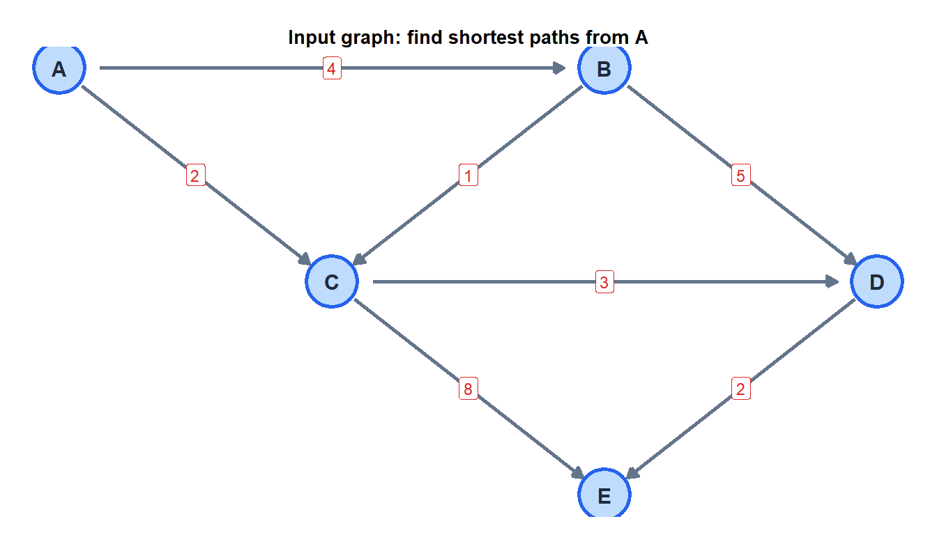
Iteration table (source = A):
| Step | Settled | \(d[A]\) | \(d[B]\) | \(d[C]\) | \(d[D]\) | \(d[E]\) |
|---|---|---|---|---|---|---|
| Init | - | 0 | \(\infty\) | \(\infty\) | \(\infty\) | \(\infty\) |
| 1 | A | 0 | 4 | 2 | \(\infty\) | \(\infty\) |
| 2 | C | 0 | 4 | 2 | 5 | 10 |
| 3 | B | 0 | 4 | 2 | 5 | 10 |
| 4 | D | 0 | 4 | 2 | 5 | 7 |
| 5 | E | 0 | 4 | 2 | 5 | 7 |
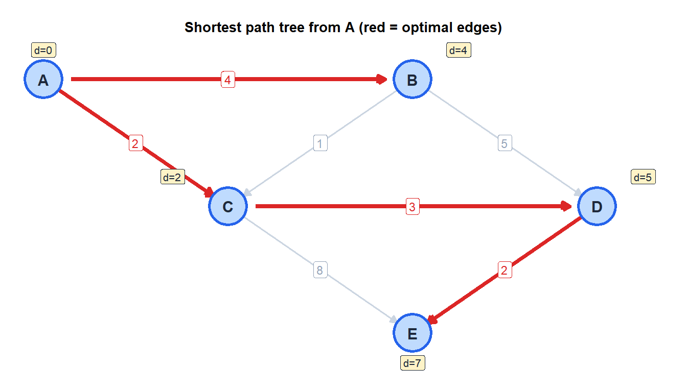
Shortest paths from A:
- A \(\to\) B: cost 4 (direct)
- A \(\to\) C: cost 2 (direct)
- A \(\to\) D: cost 5 (A-C-D)
- A \(\to\) E: cost 7 (A-C-D-E)
Complexity
The complexity depends on the priority queue implementation:
| Implementation | Extract-min | Decrease-key | Total complexity |
|---|---|---|---|
| Array (naive) | \(O(V)\) | \(O(1)\) | \(O(V^2)\) |
| Binary heap | \(O(\log V)\) | \(O(\log V)\) | \(O((V+E)\log V)\) |
| Fibonacci heap | \(O(\log V)\) | \(O(1)\) amortized | \(O(E + V\log V)\) |
For dense graphs (\(E \approx V^2\)): the array implementation is optimal at \(O(V^2)\). For sparse graphs (\(E = O(V)\) or \(O(V\log V)\)): the binary heap gives \(O(V\log V)\), much better. The Fibonacci heap is theoretically optimal but rarely used in practice due to large constants.
Most real networks (road networks, internet routing tables) are sparse, so the priority queue version is standard.
Reconstructing the shortest path
The \(\text{prev}[]\) array records the predecessor of each vertex on the shortest path. To recover the path from \(s\) to a target \(t\):
path <- c()
current <- t
while (!is.null(current)) {
  path <- c(current, path)
  current <- prev[current]
}
# path is now: s -> ... -> t
This backtracks from \(t\) to \(s\) in \(O(V)\) time.
When Dijkstra fails: negative weights
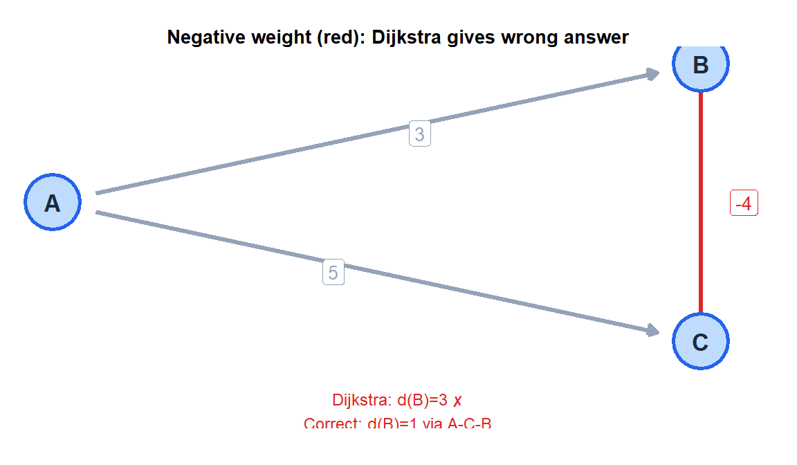
⚠️ Dijkstra's algorithm is incorrect for graphs with negative edge weights
With negative weights, settling a vertex does not guarantee its shortest distance has been found: a later path through a negative edge could be shorter. Example:
- A \(\to\) B: weight 3
- A \(\to\) C: weight 5
- C \(\to\) B: weight \(-4\)
Dijkstra settles B with distance 3. But the path A-C-B has distance \(5 + (-4) = 1 < 3\). Dijkstra never reconsiders B after settling it, so it returns the wrong answer.
For graphs with negative weights (but no negative cycles), use Bellman-Ford: \(O(VE)\) complexity, but handles negative weights correctly. For negative cycles (no shortest path exists), Bellman-Ford detects them.
Variants and extensions
| Variant | Problem | Algorithm |
|---|---|---|
| Negative weights | Shortest paths | Bellman-Ford \(O(VE)\) |
| All-pairs shortest paths | Every pair \((u,v)\) | Floyd-Warshall \(O(V^3)\) |
| Unweighted graph | Shortest path by hops | BFS \(O(V+E)\) |
| Heuristic estimate available | Single target | A* (faster in practice) |
| Dynamic graph | Edges change over time | D* or LPA* |
The A* algorithm extends Dijkstra with a heuristic function \(h(v)\) that estimates the distance from \(v\) to the target, focusing the search and reducing the number of vertices explored. It is the standard in game pathfinding and robotics.
💡 Dijkstra in R
library(igraph)

# Build the graph
g <- graph_from_data_frame(
  data.frame(from=c("A","A","B","B","C","C","D"),
             to  =c("B","C","C","D","D","E","E"),
             weight=c(4,2,1,5,3,8,2)),
  directed=TRUE
)

# Shortest distances from A
distances(g, v="A", weights=E(g)$weight)

# Shortest path from A to E (with vertex sequence)
shortest_paths(g, from="A", to="E", weights=E(g)$weight)$vpath

# All-pairs shortest paths
distances(g, weights=E(g)$weight)
