Shapley values and SHAP
Shapley values answer a deceptively simple question: given a model prediction for a specific observation, how much did each feature contribute to that prediction? They come from cooperative game theory and have a unique mathematical justification: they are the only attribution method that satisfies four natural fairness axioms simultaneously. SHAP makes Shapley values tractable for machine learning models.
The attribution problem
A model predicts that a loan applicant has a 78% probability of default, compared to the average prediction of 35%. The prediction is 43 percentage points above average. How much of that excess does each feature (income, age, credit history, debt ratio) explain?
This is not a trivial question. Features interact: the effect of income depends on the debt ratio. A naive approach that evaluates features one at a time misses these interactions. Shapley values solve this by averaging over all possible orderings in which features can be “introduced” into the model.
Shapley values: the game theory foundation
In cooperative game theory, a set of players \(N = \{1, \ldots, p\}\) play a game and earn a joint payoff \(v(S)\) for each coalition \(S \subseteq N\). The Shapley value \(\phi_j\) is the fair share of player \(j\):
\[\phi_j = \sum_{S \subseteq N \setminus \{j\}} \frac{|S|!\,(p-|S|-1)!}{p!} \left[v(S \cup \{j\}) - v(S)\right]\]
For model interpretability: players = features, payoff = model prediction, \(v(S)\) = expected model output when only features in \(S\) are known (others are marginalized out).
The formula averages the marginal contribution of feature \(j\) over all possible orderings of the features: how much does adding \(j\) to the coalition \(S\) change the prediction?
The four fairness axioms
Shapley values are the unique attribution that satisfies all four simultaneously:
Efficiency: the Shapley values sum to the difference between the prediction and the baseline (average prediction):
\[\sum_{j=1}^p \phi_j = f(\mathbf{x}) - E[f(\mathbf{X})]\]
Every deviation from the baseline is fully explained.
Symmetry: if two features \(j\) and \(k\) make identical contributions to every coalition (\(v(S \cup \{j\}) = v(S \cup \{k\})\) for all \(S\)), they receive the same Shapley value.
Dummy: if a feature \(j\) does not change the prediction in any coalition (\(v(S \cup \{j\}) = v(S)\) for all \(S\)), its Shapley value is zero.
Additivity: for models that decompose as \(f = f_1 + f_2\), the Shapley values add: \(\phi_j(f) = \phi_j(f_1) + \phi_j(f_2)\).
No other attribution method satisfies all four. Methods like gradient-based attribution, LIME, and permutation importance violate at least one axiom.
SHAP: efficient Shapley approximation
Computing exact Shapley values requires evaluating the model on all \(2^p\) subsets, which is exponential. SHAP (SHapley Additive exPlanations, Lundberg and Lee 2017) provides efficient exact or approximate algorithms for specific model classes:
TreeSHAP: exact Shapley values for tree-based models (decision trees, random forests, XGBoost, LightGBM) in \(O(TLD^2)\) time where \(T\) is the number of trees, \(L\) is the number of leaves, and \(D\) is the tree depth. This is polynomial, making it feasible for large ensembles.
LinearSHAP: exact Shapley values for linear models. For a linear model \(f(\mathbf{x}) = \boldsymbol{\beta}^T\mathbf{x} + \beta_0\), the Shapley value of feature \(j\) is simply \(\phi_j = \beta_j(x_j - E[x_j])\) when features are independent.
KernelSHAP: model-agnostic approximation using weighted linear regression on sampled coalitions. Works for any black-box model but is slower.
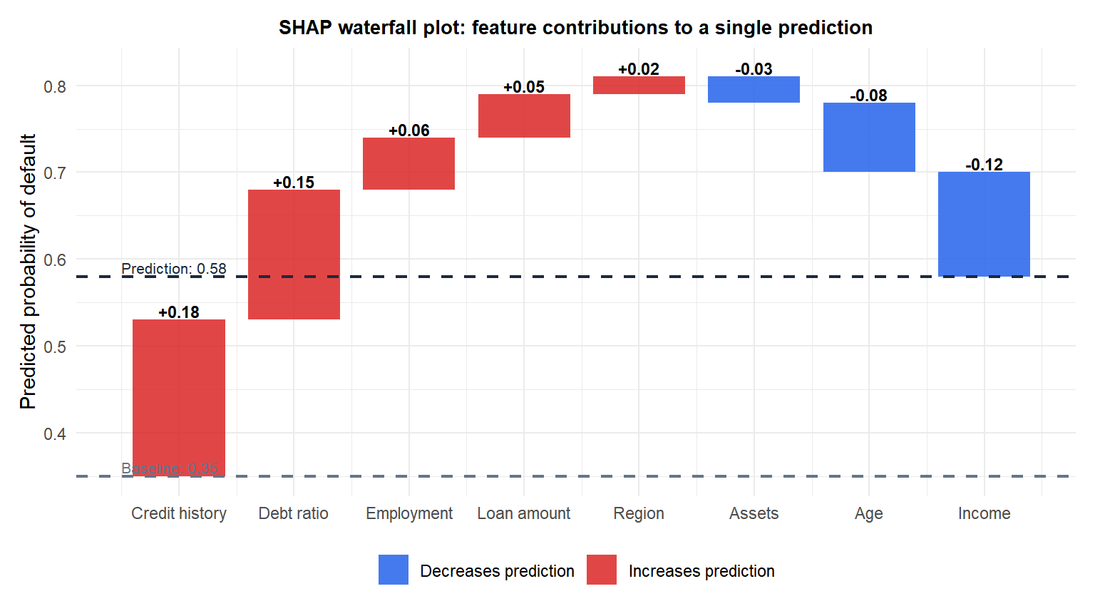
The waterfall plot starts at the baseline (average prediction = 0.35) and adds each feature’s SHAP value sequentially. Red bars push the prediction up; blue bars pull it down. The final prediction (0.58) equals the baseline plus all SHAP values, satisfying the efficiency axiom.
Global interpretability: the SHAP summary plot
Individual Shapley values explain one prediction. To understand the model globally, compute SHAP values for all observations and visualize the distribution.
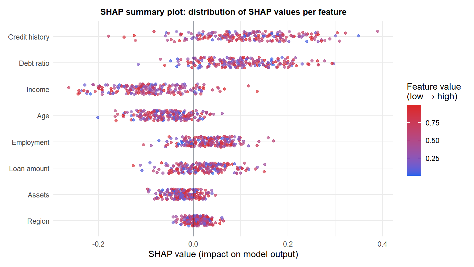
Each dot is one observation. Position on x shows the SHAP value (direction and magnitude of the feature’s effect). Color shows the feature value (blue = low, red = high). The summary plot reveals: high debt ratio (red) pushes predictions up; high income (red) pushes predictions down. Features are ordered by mean absolute SHAP value (global importance).
SHAP vs traditional feature importance
| Permutation importance | Impurity importance | SHAP | |
|---|---|---|---|
| Explains individual predictions | No | No | Yes |
| Consistent with model | No (may differ) | No | Yes (efficiency axiom) |
| Handles correlated features | Poorly | Poorly | Better |
| Shows direction of effect | No | No | Yes |
| Computationally expensive | Moderate | Fast | Fast (TreeSHAP) |
SHAP dominates traditional feature importance in almost every dimension except speed (though TreeSHAP is fast enough for most applications). For correlated features, SHAP distributes credit more fairly than permutation importance, which can assign zero importance to a relevant feature if a correlated feature absorbs its effect.
⚠️ SHAP measures association, not causation
A SHAP value of +0.18 for “credit history” means that knowing the credit history of this applicant pushes the model’s prediction 18 percentage points above the baseline. It does not mean that changing the credit history would change the outcome by 18 percentage points in the real world.
SHAP explains the model, not the data-generating process. If the model has learned a spurious correlation (e.g., zip code as a proxy for race in a biased dataset), SHAP will dutifully explain that spurious association. Interpretability tools make models more transparent; they do not make flawed models correct.
Also: SHAP values depend on the reference distribution used to marginalize out missing features. Different implementations handle this differently (marginal vs conditional expectation), leading to different values for the same model. Always check which baseline is being used.
💡 SHAP in R
library(shapviz)   # best SHAP visualization in R
library(xgboost)

# Train XGBoost model
dtrain <- xgb.DMatrix(X_train, label=y_train)
fit <- xgb.train(params=list(eta=0.1, max_depth=5,
                              objective="binary:logistic"),
                 data=dtrain, nrounds=100)

# Compute exact SHAP values (TreeSHAP)
shp <- shapviz(fit, X_pred=X_train)

# Waterfall plot for one observation
sv_waterfall(shp, row_id=1)

# Summary (beeswarm) plot
sv_importance(shp, kind="beeswarm")

# Dependence plot: SHAP vs feature value for one feature
sv_dependence(shp, v="income")

# Mean absolute SHAP (global importance bar chart)
sv_importance(shp, kind="bar")

# For any black-box model: KernelSHAP
library(kernelshap)
ks <- kernelshap(fit_rf, X=X_train, bg_X=X_train[1:100,])
sv <- shapviz(ks)
sv_importance(sv, kind="beeswarm")
