Ridge regression
Ridge regression (also called Tikhonov regularization or \(L_2\) regularization) adds the sum of squared coefficients as a penalty to the OLS objective. The result is a closed-form solution that shrinks all coefficients toward zero and fixes the instability caused by near-singular or singular design matrices.
Objective function and solution
\[\hat{\boldsymbol{\beta}}^R = \arg\min_{\boldsymbol{\beta}} \|\mathbf{y} - \mathbf{X}\boldsymbol{\beta}\|_2^2 + \lambda\|\boldsymbol{\beta}\|_2^2\]
\[\hat{\boldsymbol{\beta}}^R = (\mathbf{X}^T\mathbf{X} + \lambda\mathbf{I})^{-1}\mathbf{X}^T\mathbf{y}\]
Adding \(\lambda\mathbf{I}\) to \(\mathbf{X}^T\mathbf{X}\) before inverting is the key operation. Even when \(\mathbf{X}^T\mathbf{X}\) is singular (perfectly collinear predictors, \(p > n\)), \(\mathbf{X}^T\mathbf{X} + \lambda\mathbf{I}\) is always invertible for any \(\lambda > 0\). This is why Ridge is particularly effective for multicollinearity.
The bias-variance decomposition of the Ridge estimator:
\[E[\hat{\boldsymbol{\beta}}^R] = (\mathbf{X}^T\mathbf{X} + \lambda\mathbf{I})^{-1}\mathbf{X}^T\mathbf{X}\boldsymbol{\beta} \neq \boldsymbol{\beta} \quad (\text{biased})\]
\[\text{Var}(\hat{\boldsymbol{\beta}}^R) = \sigma^2(\mathbf{X}^T\mathbf{X} + \lambda\mathbf{I})^{-1}\mathbf{X}^T\mathbf{X}(\mathbf{X}^T\mathbf{X} + \lambda\mathbf{I})^{-1}\]
The variance is strictly smaller than OLS variance; the bias increases with \(\lambda\). For sufficiently large \(\lambda\), the reduction in variance outweighs the increase in bias: total MSE decreases.
SVD interpretation: shrinking the singular values
The singular value decomposition \(\mathbf{X} = \mathbf{U}\mathbf{D}\mathbf{V}^T\) (with singular values \(d_1 \geq d_2 \geq \cdots \geq d_p\)) gives a clean picture of what Ridge does:
\[\hat{\boldsymbol{\beta}}^R = \mathbf{V}\text{diag}\!\left(\frac{d_j^2}{d_j^2 + \lambda}\right)\mathbf{V}^T\hat{\boldsymbol{\beta}}^{\text{OLS}}\]
Each coefficient is multiplied by a shrinkage factor \(d_j^2/(d_j^2 + \lambda) \in (0,1)\). Directions with large singular values (high variance, well-determined by data) are shrunk little. Directions with small singular values (low variance, poorly determined, associated with near-collinear predictors) are shrunk heavily.
Ridge does not eliminate any direction: it shrinks all of them, more aggressively in the directions where the data provides least information.
Ridge and multicollinearity
Multicollinearity inflates the variance of OLS coefficients because \(\mathbf{X}^T\mathbf{X}\) is nearly singular: small eigenvalues produce enormous entries in \((\mathbf{X}^T\mathbf{X})^{-1}\). Adding \(\lambda\mathbf{I}\) raises all eigenvalues by \(\lambda\), dramatically reducing \((\mathbf{X}^T\mathbf{X} + \lambda\mathbf{I})^{-1}\) in the near-zero eigenvalue directions.
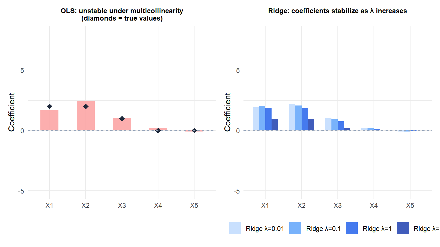
OLS (left) produces wildly unstable coefficients for \(X_1\) and \(X_2\) (nearly collinear). Ridge (right) progressively stabilizes them as \(\lambda\) increases, converging toward equal and stable estimates.
Shrinkage path and effective df
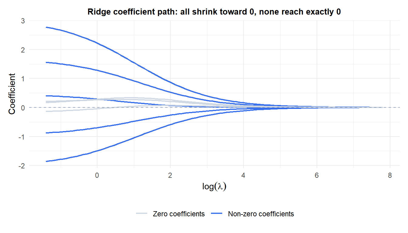
All coefficients shrink smoothly as \(\lambda\) increases. The five truly nonzero coefficients (blue) persist longer; the zero ones (grey) were already near zero. None of them ever reach exactly zero, which distinguishes Ridge from Lasso.
The effective degrees of freedom of the Ridge fit:
\[\text{df}(\lambda) = \text{tr}\left[\mathbf{X}(\mathbf{X}^T\mathbf{X} + \lambda\mathbf{I})^{-1}\mathbf{X}^T\right] = \sum_{j=1}^p \frac{d_j^2}{d_j^2 + \lambda}\]
At \(\lambda=0\): df = \(p\) (OLS). As \(\lambda \to \infty\): df \(\to\) 0. This provides an interpretable measure of model complexity.
When to use Ridge
Ridge is the natural choice when:
- Predictors are highly correlated (multicollinearity).
- \(p\) is large relative to \(n\) but all predictors are expected to contribute (dense signal).
- The goal is prediction accuracy rather than variable selection.
- The relationship between response and predictors is known to be dense (many small effects rather than a few large ones).
If the true model is sparse (only a few predictors matter), Lasso or ElasticNet will outperform Ridge because they set irrelevant coefficients to exactly zero.
⚠️ Ridge does not perform variable selection
A common mistake: fitting Ridge and then using the non-zero coefficients as a selected subset of predictors. Every Ridge coefficient is nonzero for any finite \(\lambda\). If you need to know which predictors matter, use Lasso or ElasticNet. Ridge gives you a prediction model, not a variable selection tool.
💡 Ridge regression in R
library(glmnet)

# Fit Ridge (alpha=0)
fit_ridge <- glmnet(X, y, alpha=0)
plot(fit_ridge, xvar="lambda", label=TRUE)  # coefficient path

# Select lambda by 10-fold CV
cv_ridge <- cv.glmnet(X, y, alpha=0, nfolds=10)
plot(cv_ridge)
best_lambda <- cv_ridge$lambda.min

# Coefficients and predictions
coef(cv_ridge, s="lambda.min")
predict(cv_ridge, newx=X_new, s="lambda.min")

# Effective degrees of freedom
d <- svd(X)$d
df_lambda <- sum(d^2 / (d^2 + best_lambda))
