Regularization
Regularization adds a penalty on the size of model coefficients to the loss function. This shrinks the coefficients toward zero, reducing variance at the cost of a small increase in bias. The result is a model that generalizes better to new data. Ridge and Lasso are the two fundamental regularization methods; ElasticNet combines them.
Why regularization is needed
OLS minimizes the training error with no constraint on coefficient size. When the number of predictors \(p\) is large relative to \(n\), or when predictors are correlated, OLS produces large, unstable coefficients that fit the training data well but fail on new data.
Consider fitting a model with \(p = n - 1\) predictors: OLS achieves zero training error by interpolating every point. The coefficients are enormous and the model is useless for prediction. Regularization prevents this by penalizing large coefficients.
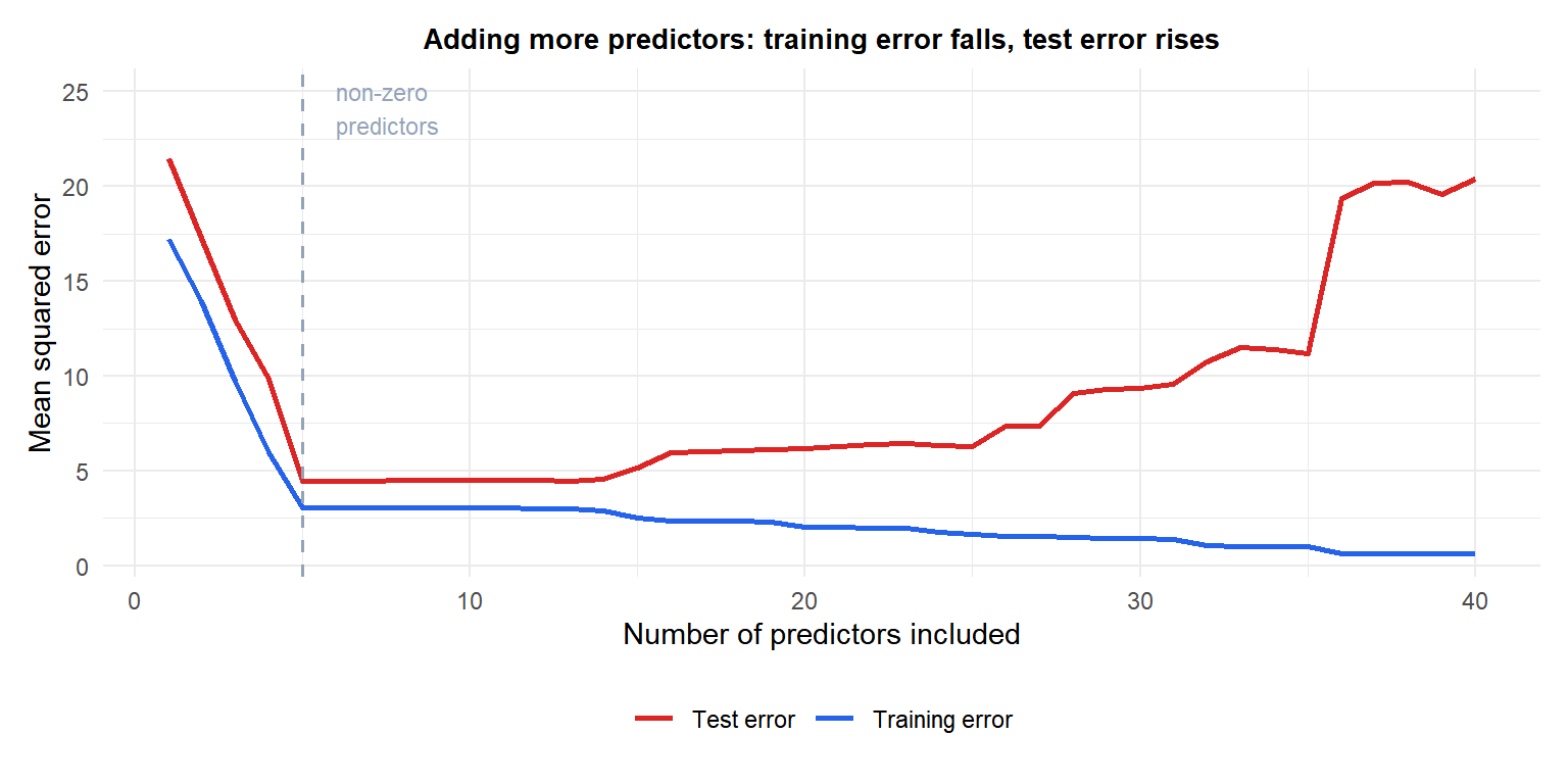
Training error (blue) always decreases as more predictors are added. Test error (red) decreases initially, then rises as the model starts overfitting noise.
The penalized loss framework
Regularization modifies the OLS objective by adding a penalty on the coefficient vector:
\[\hat{\boldsymbol{\beta}}_\lambda = \arg\min_{\boldsymbol{\beta}} \underbrace{\|\mathbf{y} - \mathbf{X}\boldsymbol{\beta}\|_2^2}_{\text{data fit}} + \lambda \underbrace{\Omega(\boldsymbol{\beta})}_{\text{penalty}}\]
- \(\lambda \geq 0\): the regularization parameter. Controls the strength of the penalty.
- \(\lambda = 0\): no regularization, reduces to OLS.
- \(\lambda \to \infty\): all coefficients shrink to zero.
- \(\Omega(\boldsymbol{\beta})\): the penalty function. Different choices give different methods.
The intercept \(\beta_0\) is never penalized: it only shifts the predictions and shrinking it would introduce bias in the mean.
Ridge (\(L_2\)) and Lasso (\(L_1\))
Ridge regression (\(L_2\) penalty)
\[\hat{\boldsymbol{\beta}}^{\text{Ridge}} = \arg\min_{\boldsymbol{\beta}} \|\mathbf{y} - \mathbf{X}\boldsymbol{\beta}\|_2^2 + \lambda \sum_j \beta_j^2\]
Has a closed-form solution: \(\hat{\boldsymbol{\beta}}^{\text{Ridge}} = (\mathbf{X}^T\mathbf{X} + \lambda\mathbf{I})^{-1}\mathbf{X}^T\mathbf{y}\).
Ridge shrinks all coefficients toward zero but never to exactly zero. It handles multicollinearity well: adding \(\lambda\mathbf{I}\) makes \(\mathbf{X}^T\mathbf{X} + \lambda\mathbf{I}\) invertible even when \(\mathbf{X}^T\mathbf{X}\) is singular.
Lasso regression (\(L_1\) penalty)
\[\hat{\boldsymbol{\beta}}^{\text{Lasso}} = \arg\min_{\boldsymbol{\beta}} \|\mathbf{y} - \mathbf{X}\boldsymbol{\beta}\|_2^2 + \lambda \sum_j |\beta_j|\]
No closed-form solution: requires coordinate descent or subgradient methods. The key property: Lasso can shrink coefficients to exactly zero, performing automatic variable selection. Coefficients of irrelevant predictors are set to exactly zero as \(\lambda\) increases.
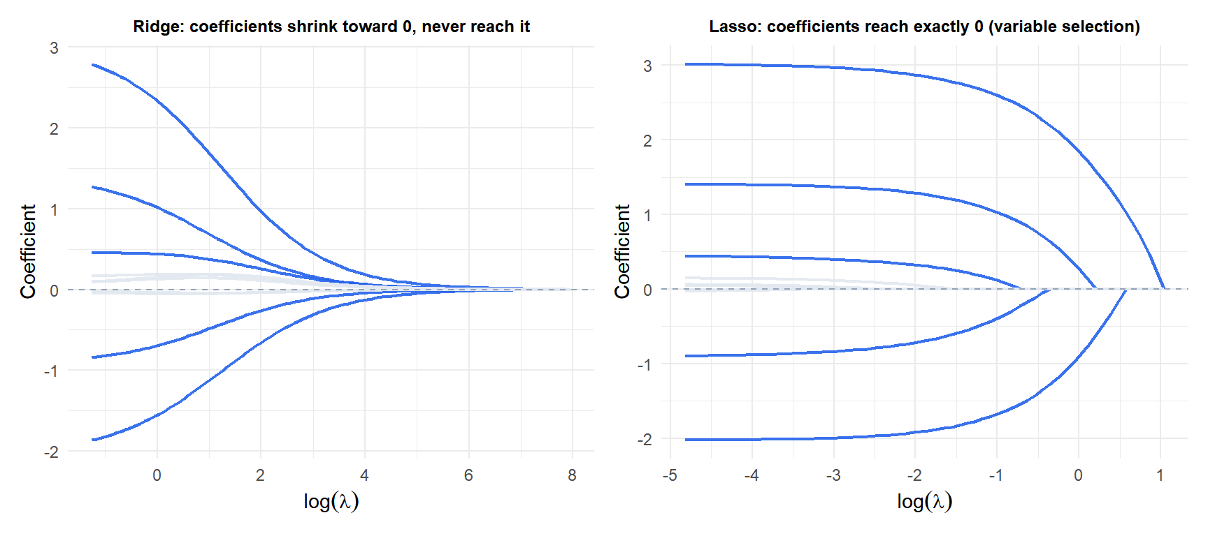
In the Ridge path (left), all coefficients shrink smoothly but remain nonzero. In the Lasso path (right), the five truly zero coefficients (grey) are eliminated early as \(\lambda\) increases; the five nonzero ones (blue) persist longer.
Geometric intuition
The constrained form of regularization reveals why the two penalties behave differently:
- Ridge: minimize \(\|\mathbf{y}-\mathbf{X}\boldsymbol{\beta}\|^2\) subject to \(\sum_j \beta_j^2 \leq t\). The constraint region is a sphere. The OLS solution is pulled toward the sphere surface; it touches the sphere at a point where no coefficient is exactly zero.
- Lasso: minimize subject to \(\sum_j |\beta_j| \leq t\). The constraint region is a diamond (L1 ball). The diamond has corners on the coordinate axes. The OLS solution is pulled toward the nearest point on the diamond; it frequently hits a corner, where one or more coordinates are exactly zero.
This geometric argument explains why Lasso produces sparse solutions and Ridge does not.
Selecting \(\lambda\)
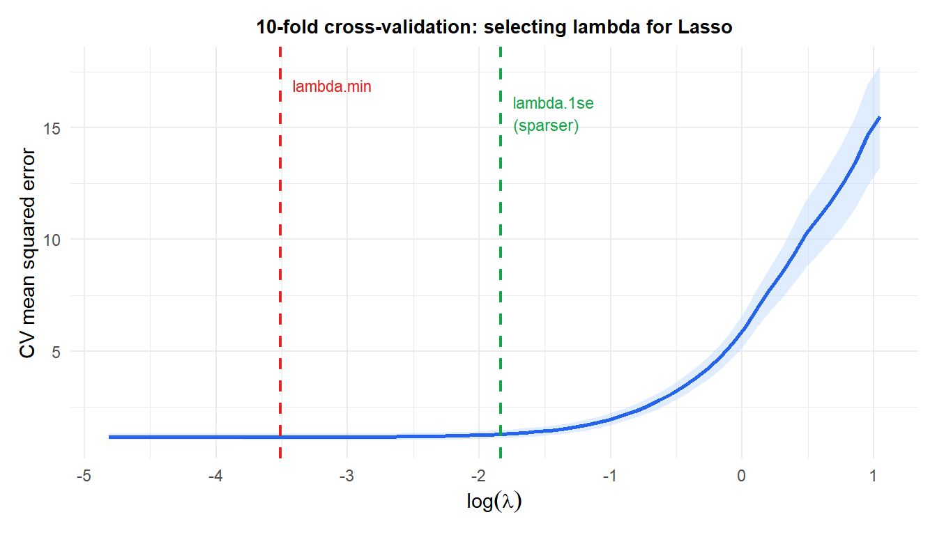
\(\lambda\) is a hyperparameter: it is not estimated from the data by OLS but selected by cross-validation. The standard approach:
- Fit the model on a grid of \(\lambda\) values (e.g., 100 values on a log scale from very large to near zero).
- For each \(\lambda\), compute the cross-validation error (typically 10-fold CV).
- Choose the \(\lambda\) that minimizes CV error (
lambda.min), or the largest \(\lambda\) within one standard error of the minimum (lambda.1se): the latter gives a sparser model with similar predictive performance.
Bayesian interpretation
Regularization has a clean Bayesian interpretation as MAP (maximum a posteriori) estimation with different priors on \(\boldsymbol{\beta}\):
- Ridge: equivalent to a Gaussian prior \(\beta_j \sim N(0, 1/\lambda)\). The Gaussian prior has no mass at exactly zero, so Ridge never produces exact sparsity.
- Lasso: equivalent to a Laplace (double exponential) prior \(\beta_j \sim \text{Laplace}(0, 1/\lambda)\). The Laplace prior has a sharp peak at zero, encouraging exact zeros.
This explains why Lasso does variable selection and Ridge does not: it is a consequence of the shape of the prior at zero.
⚠️ Standardize predictors before regularizing
Ridge and Lasso penalize large coefficients. If the predictors are on different scales (e.g., income in thousands vs. age in years), the penalties are applied unequally: the predictor with the largest scale gets the most shrinkage regardless of its importance.
Always standardize predictors to zero mean and unit variance before fitting regularized models. glmnet does this automatically by default (standardize=TRUE). When using other software, standardize manually first.
Also: the intercept is not penalized and should not be standardized.
💡 Ridge and Lasso in R
library(glmnet)

# Standardize predictors (done automatically by glmnet)
# alpha=0: Ridge; alpha=1: Lasso; alpha in (0,1): ElasticNet
fit_ridge <- glmnet(X, y, alpha=0)
fit_lasso <- glmnet(X, y, alpha=1)

# Select lambda by cross-validation
cv_fit <- cv.glmnet(X, y, alpha=1, nfolds=10)
best_lambda <- cv_fit$lambda.min     # minimum CV error
sparse_lambda <- cv_fit$lambda.1se  # 1-SE rule (sparser)

# Coefficients at best lambda
coef(cv_fit, s="lambda.min")
coef(cv_fit, s="lambda.1se")

# Predictions
predict(cv_fit, newx=X_new, s="lambda.min")
