Linear regression diagnostics
Regression diagnostics check whether the assumptions behind OLS are satisfied and whether any observations unduly distort the model. Running a regression without diagnostics is like accepting a result without checking the work: the estimates may be correct, or they may be completely wrong, and you cannot tell which without looking.
The LINE assumptions
The four assumptions of linear regression, remembered as LINE:
- Linearity: \(E[y|x] = \mathbf{x}^T\boldsymbol{\beta}\) (the conditional mean is linear in the predictors).
- Independence: residuals \(\varepsilon_i\) are independent across observations.
- Normality: \(\varepsilon_i \sim N(0, \sigma^2)\).
- Equal variance (homoscedasticity): \(\text{Var}(\varepsilon_i) = \sigma^2\) for all \(i\).
Linearity and independence are the critical ones: violations lead to biased or inconsistent estimates. Normality matters mainly for small samples (inference is robust to non-normality for large \(n\) via CLT). Heteroscedasticity does not bias \(\hat{\boldsymbol{\beta}}\) but inflates or deflates standard errors, making hypothesis tests unreliable.
The four diagnostic plots
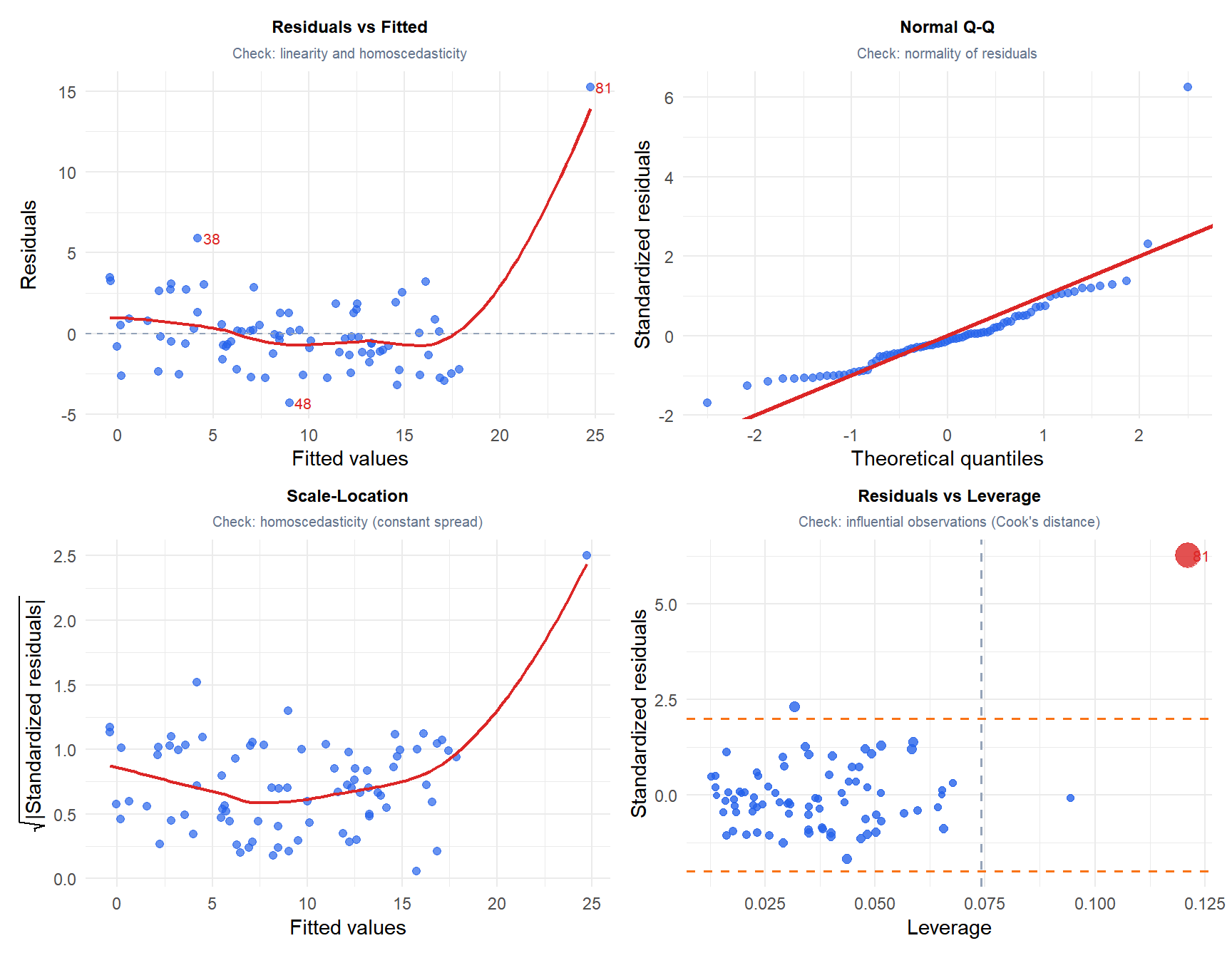
The four plots expose different assumption violations:
- Residuals vs Fitted: a flat red line means linearity holds. A U-shape or funnel indicates non-linearity or heteroscedasticity.
- Normal Q-Q: points on the diagonal mean normality holds. S-shaped curves indicate heavy tails; curved departures indicate skewness.
- Scale-Location: a flat red line means homoscedasticity holds. An upward trend means variance increases with the fitted value.
- Residuals vs Leverage: points with high Cook’s distance (large bubbles, labeled) are influential. The dashed horizontal lines mark \(\pm 2\) standardized residuals.
Formal tests for assumption violations
Breusch-Pagan test for heteroscedasticity
Regresses the squared residuals on the predictors. A significant result rejects \(H_0\): constant variance.
Shapiro-Wilk test for residual normality
Tests whether the residuals come from a normal distribution. For large \(n\) (\(> 5{,}000\)), even trivial non-normality is detected: use Q-Q plots to assess practical significance.
Durbin-Watson test for autocorrelation
\[DW = \frac{\sum_{i=2}^n (e_i - e_{i-1})^2}{\sum_{i=1}^n e_i^2}\]
\(DW \approx 2\) means no autocorrelation. \(DW < 1.5\) suggests positive autocorrelation (consecutive residuals tend to have the same sign). Relevant for time series data; less important for cross-sectional data.
Outliers, leverage and influential points
Three distinct concepts that are often confused:
Outlier
A point with a large residual: the observed \(y_i\) is far from \(\hat{y}_i\). Detected by standardized residuals \(|e_i / \hat{\sigma}| > 2\) or \(> 3\). An outlier in \(y\) does not necessarily influence the regression line if its \(x_i\) is near \(\bar{x}\).
High leverage
A point with an extreme value of \(x_i\), far from the center of the predictor space. Measured by the hat matrix diagonal \(h_{ii} = \mathbf{x}_i^T(\mathbf{X}^T\mathbf{X})^{-1}\mathbf{x}_i\). A common threshold is \(h_{ii} > 2(k+1)/n\). High leverage points have the potential to influence the fit, but may or may not do so depending on their \(y_i\) value.
Influential point
A point that actually changes the regression coefficients substantially when removed. Combines high leverage with a large residual. Measured by Cook’s distance:
\[D_i = \frac{(\hat{\boldsymbol{\beta}} - \hat{\boldsymbol{\beta}}_{(-i)})^T \mathbf{X}^T\mathbf{X} (\hat{\boldsymbol{\beta}} - \hat{\boldsymbol{\beta}}_{(-i)})}{(k+1)\hat{\sigma}^2}\]
\(D_i > 0.5\) warrants investigation; \(D_i > 1\) is generally considered influential.
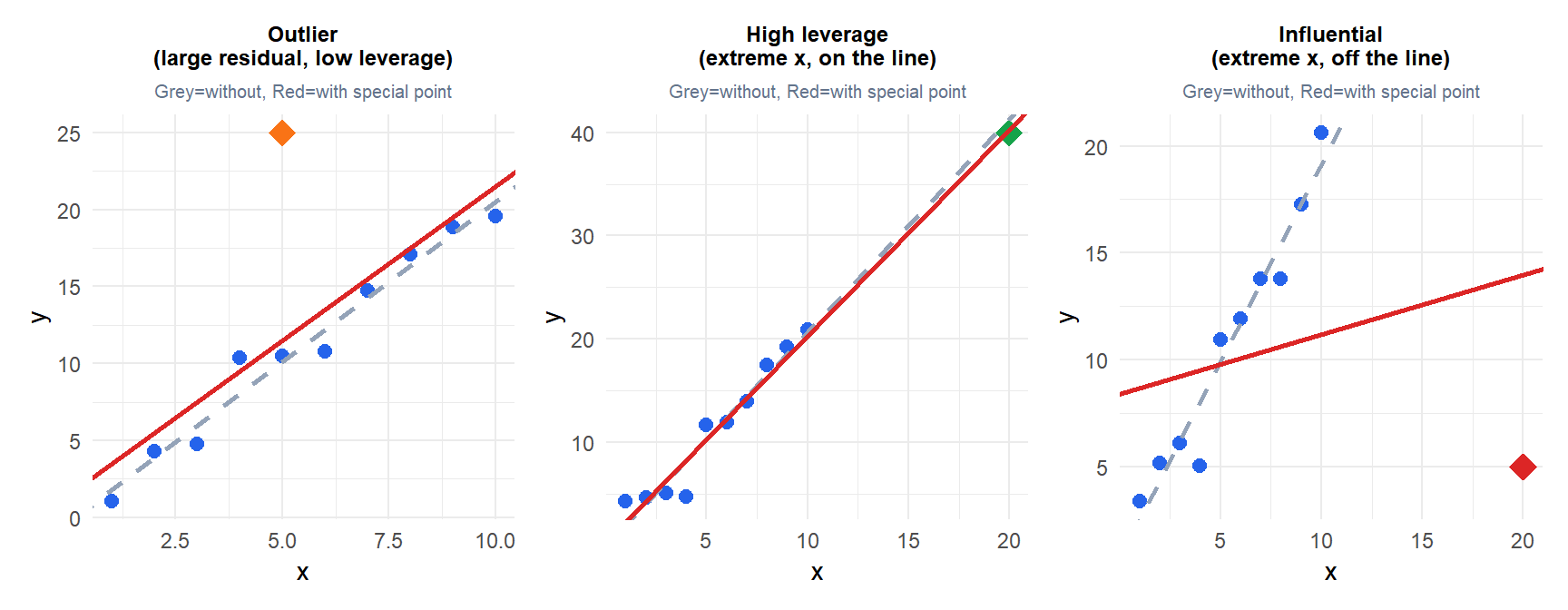
The outlier (orange) has a large residual but sits at \(x=5\) (near \(\bar{x}\)): the line barely moves. The high leverage point (green) is far from \(\bar{x}\) but lies on the true line: the line barely moves. The influential point (red) combines extreme \(x\) with a large residual: the line rotates substantially.
⚠️ Never delete influential points without investigation
An influential observation is not automatically an error. It could be:
- A genuine extreme but valid data point that the model should accommodate.
- A data entry error that should be corrected.
- A structural break or special event (a financial crisis, a policy change) that warrants a separate indicator variable.
Before removing any point, investigate why it is influential. Deleting valid influential observations to improve fit metrics is data manipulation and produces a model that will fail on similar observations in the future.
💡 Regression diagnostics in R
fit <- lm(y ~ x1 + x2, data=df)

# Four diagnostic plots at once
par(mfrow=c(2,2))
plot(fit)

# Formal tests
library(lmtest)
bptest(fit)          # Breusch-Pagan: H0 = homoscedasticity
dwtest(fit)          # Durbin-Watson: H0 = no autocorrelation
shapiro.test(residuals(fit))   # H0 = normality

# Influence measures
influencePlot(fit)   # leverage vs standardized residuals
cooks.distance(fit)
hatvalues(fit)

# All at once
library(car)
outlierTest(fit)     # Bonferroni-corrected test for outliers
vif(fit)             # multicollinearity
