Random forest
Random forest builds a large number of deep decision trees on bootstrap samples of the data, using a random subset of features at each split. The final prediction is the majority vote (classification) or average (regression) across all trees. Averaging many decorrelated trees dramatically reduces variance while leaving bias essentially unchanged, making random forest one of the most reliable off-the-shelf algorithms in machine learning.
From a single tree to bagging
A single decision tree has low bias but high variance: small changes in the training data can produce a completely different tree. The key insight behind bagging (bootstrap aggregating): if we average many independent unbiased estimators, the variance of the average is \(\sigma^2/B\) where \(B\) is the number of estimators.
For \(B\) trees each with variance \(\sigma^2\) and pairwise correlation \(\rho\), the variance of the average is:
\[\text{Var}\!\left(\frac{1}{B}\sum_{b=1}^B \hat{f}_b(\mathbf{x})\right) = \rho\sigma^2 + \frac{1-\rho}{B}\sigma^2\]
As \(B \to \infty\), the second term vanishes. The remaining variance is \(\rho\sigma^2\): the correlation between trees sets a floor on how much bagging can help. Trees trained on bootstrap samples of the same data are correlated (they all use the same strong predictors), so bagging alone leaves substantial variance.
Random forest’s innovation: at each split, only a random subset of \(m\) features is considered (instead of all \(p\)). This prevents strong predictors from dominating every tree, decorrelating the ensemble and reducing \(\rho\).
- Classification: \(m = \lfloor\sqrt{p}\rfloor\) (default)
- Regression: \(m = \lfloor p/3 \rfloor\) (default)
The algorithm
For \(b = 1, \ldots, B\):
- Draw a bootstrap sample \(\mathcal{D}^*_b\) of size \(n\) from the training data (with replacement).
- Grow a deep decision tree on \(\mathcal{D}^*_b\). At each node, select \(m\) features at random and split on the best among those \(m\).
- Do not prune.
For a new point \(\mathbf{x}\):
\[\hat{f}^{RF}(\mathbf{x}) = \frac{1}{B}\sum_{b=1}^B \hat{f}_b(\mathbf{x}) \quad \text{(regression)}\]
\[\hat{c}^{RF}(\mathbf{x}) = \text{majority vote}\{c_b(\mathbf{x})\}_{b=1}^B \quad \text{(classification)}\]
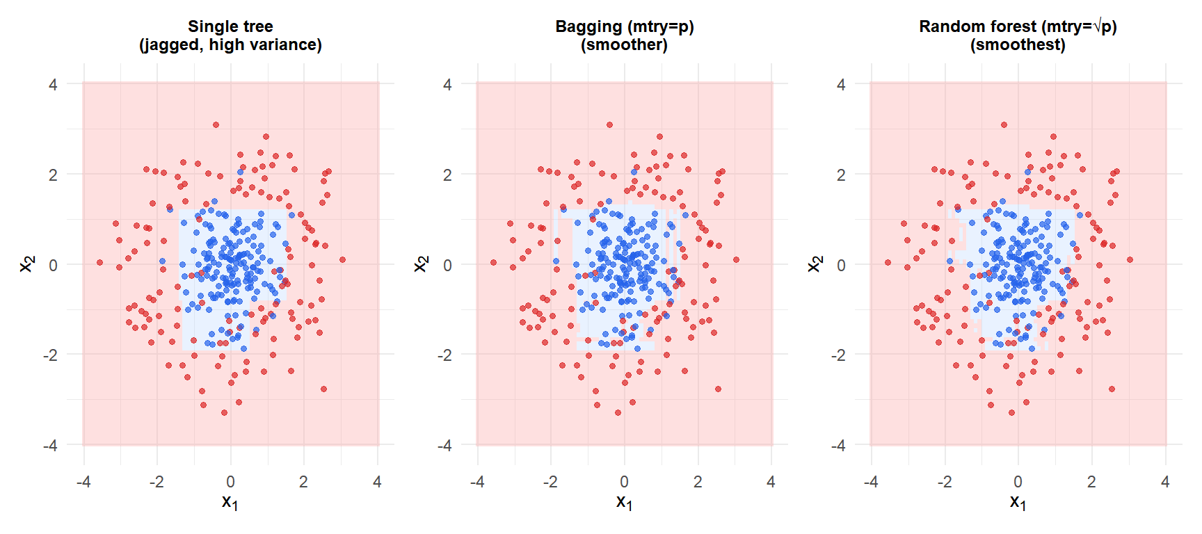
The single tree (left) has an irregular boundary that follows noise. Bagging (centre) smooths it but correlated trees limit the improvement. Random forest (right) produces the smoothest boundary by decorrelating the trees through feature subsampling.
Out-of-bag error
Each bootstrap sample omits approximately \(1/e \approx 37\%\) of the training observations (the out-of-bag observations). Tree \(b\) was not trained on its OOB observations, so they can be used as a validation set:
\[\hat{f}^{OOB}(\mathbf{x}_i) = \frac{1}{|\{b: i \in \text{OOB}_b\}|} \sum_{b: i \in \text{OOB}_b} \hat{f}_b(\mathbf{x}_i)\]
The OOB error averages the prediction errors over all training points using only trees that did not see that point. It is a nearly unbiased estimate of the test error, without requiring a separate validation set.
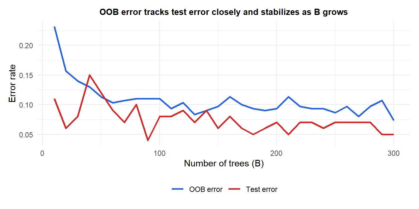
OOB error (blue) closely tracks the true test error (red) without requiring a separate validation set. Both stabilize after roughly 100-200 trees: adding more trees beyond this point does not improve accuracy but does increase computation time.
Feature importance
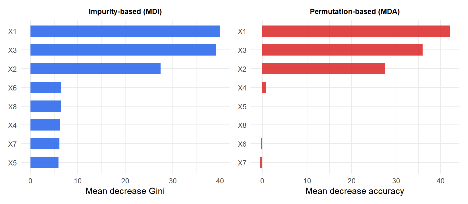
Impurity-based importance (mean decrease in impurity)
The importance of feature \(j\) is the total decrease in node impurity weighted by the proportion of samples reaching each node, averaged across all trees:
\[\text{MDI}(j) = \frac{1}{B}\sum_{b=1}^B \sum_{\text{nodes on } j \text{ in tree } b} \frac{n_\text{node}}{n} \cdot \Delta G\]
Fast to compute. Biased toward high-cardinality features: features with many unique values have more split opportunities and tend to score higher even if not truly important.
Permutation importance (mean decrease in accuracy)
For each feature \(j\): permute its values in the OOB samples (breaking the association with the response), re-predict, and measure the increase in OOB error. Features that matter will cause large error increases when permuted:
\[\text{MDA}(j) = \frac{1}{B}\sum_{b=1}^B \left[\text{OOB error after permuting } j \text{ in tree } b\right] - \text{OOB error}\]
More reliable than impurity-based importance: not biased by cardinality, measures actual predictive contribution rather than tree structure.
Key hyperparameters
| Parameter | Default | Effect |
|---|---|---|
ntree (\(B\)) |
500 | More trees = lower variance, diminishing returns after ~200 |
mtry (\(m\)) |
\(\sqrt{p}\) / \(p/3\) | Lower \(m\) = more decorrelated trees, higher individual bias |
maxdepth |
None (full) | Shallower trees = higher bias, lower variance |
nodesize |
1 (class) / 5 (reg) | Minimum node size before splitting |
mtry is the most important hyperparameter. Tune it with OOB error: try values from 1 to \(p\) and choose the one with lowest OOB error.
⚠️ Random forest feature importance can be misleading with correlated features
When two features are highly correlated, permuting one does not eliminate its information (the other feature carries it). Both features may appear unimportant even if the pair collectively has high predictive power. Conversely, impurity-based importance splits the credit arbitrarily between them.
For reliable importance estimates with correlated features: use conditional permutation importance (permimp package), which conditions on the values of correlated features when permuting. Or use SHAP values (treeshap package) which provide consistent, theoretically grounded attributions.
💡 Random forest in R
library(randomForest)

# Classification
fit <- randomForest(y ~ ., data=df_train,
                    ntree=500, mtry=floor(sqrt(ncol(df_train)-1)),
                    importance=TRUE)

# OOB error evolution
plot(fit)   # error rate vs number of trees

# Feature importance
importance(fit)
varImpPlot(fit)

# Tune mtry with OOB error
library(caret)
ctrl <- trainControl(method="oob")
fit_cv <- train(y ~ ., data=df_train, method="rf",
                trControl=ctrl,
                tuneGrid=data.frame(mtry=c(1,2,3,5,8)))
fit_cv$bestTune

# Regression forest
fit_reg <- randomForest(y ~ ., data=df_train, ntree=500)
fit_reg$mse   # OOB MSE per tree
