Neural networks

A feedforward neural network is a composition of affine transformations and nonlinear activation functions. Adding layers allows the network to learn hierarchical representations: early layers detect simple patterns, later layers combine them into complex ones. Backpropagation efficiently computes the gradient of the loss with respect to every weight via the chain rule, enabling gradient descent to optimize millions of parameters.

Architecture

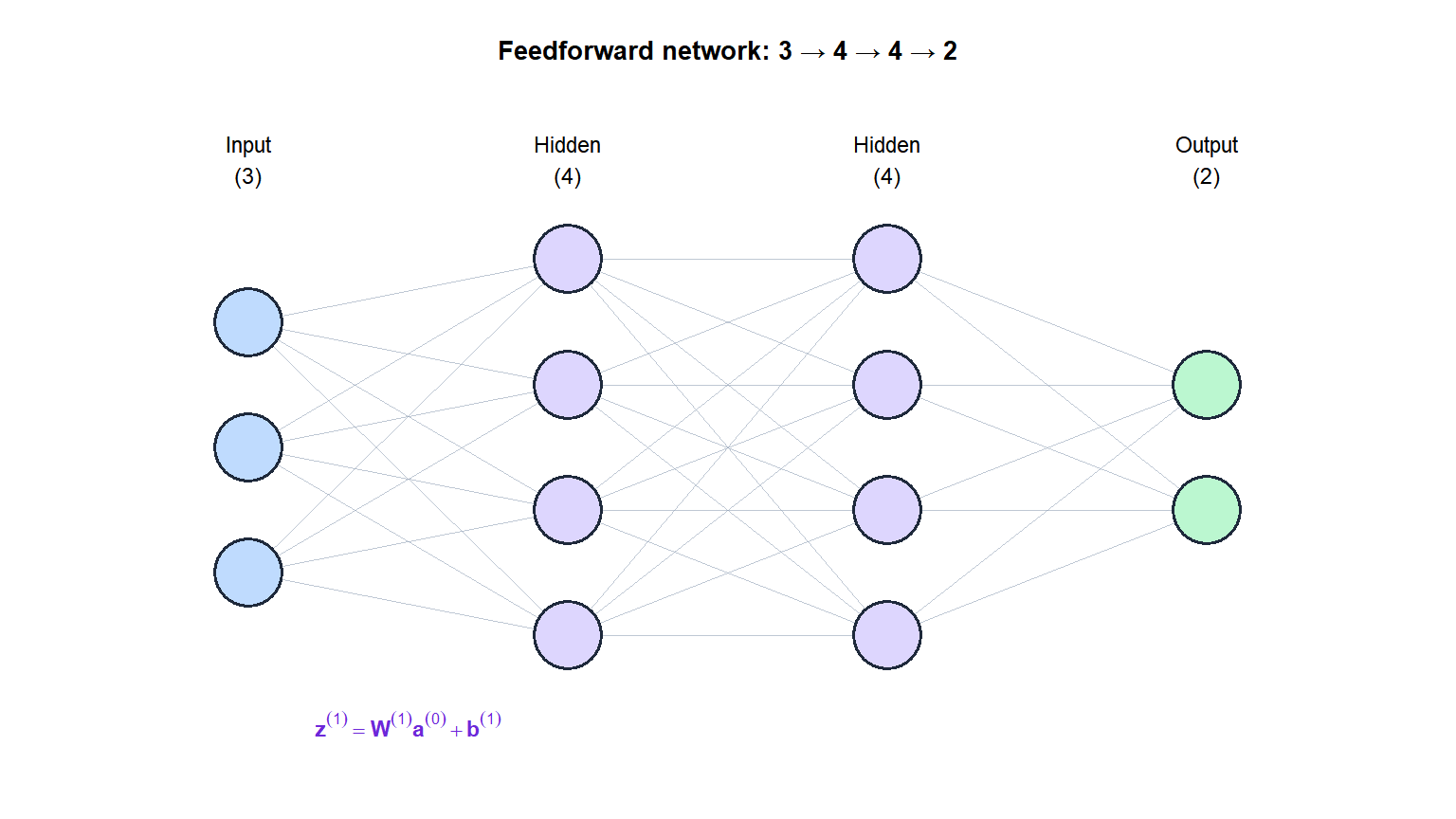
A network with \(L\) layers computes:

\[\mathbf{a}^{(0)} = \mathbf{x} \quad (\text{input})\]

\[\mathbf{z}^{(\ell)} = \mathbf{W}^{(\ell)}\mathbf{a}^{(\ell-1)} + \mathbf{b}^{(\ell)}, \qquad \mathbf{a}^{(\ell)} = g^{(\ell)}(\mathbf{z}^{(\ell)}), \qquad \ell = 1,\ldots,L\]

where \(\mathbf{W}^{(\ell)}\) and \(\mathbf{b}^{(\ell)}\) are the weight matrix and bias vector of layer \(\ell\), and \(g^{(\ell)}\) is the activation function. The final layer output \(\mathbf{a}^{(L)}\) is the prediction.

Universal approximation theorem: a feedforward network with a single hidden layer and a nonlinear activation can approximate any continuous function on a compact domain to arbitrary precision, given enough neurons. This guarantees expressive power but says nothing about how to find the weights or how many neurons are needed in practice.

Activation functions

Without nonlinear activation functions, a deep network collapses to a single linear transformation regardless of depth. Activation functions break this linearity.

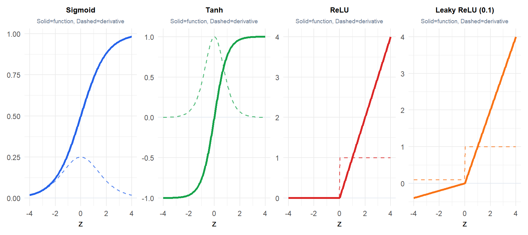
Sigmoid and tanh saturate at extreme values: their derivatives approach zero, causing the vanishing gradient problem. ReLU (\(\max(0,z)\)) has a constant derivative of 1 for positive inputs, which prevents vanishing gradients and is the default choice for hidden layers. Its weakness: dead neurons (ReLU output is always zero for inputs \(\leq 0\), so the gradient is zero and the neuron never updates). Leaky ReLU fixes this by allowing a small negative slope.

Backpropagation

Backpropagation computes \(\partial \mathcal{L}/\partial \mathbf{W}^{(\ell)}\) for all layers efficiently using the chain rule. Define the error signal at layer \(\ell\) as \(\boldsymbol{\delta}^{(\ell)} = \partial \mathcal{L}/\partial \mathbf{z}^{(\ell)}\).

Forward pass: compute \(\mathbf{z}^{(\ell)}\) and \(\mathbf{a}^{(\ell)}\) for all layers, storing intermediate values.

Backward pass: starting from the output layer:

\[\boldsymbol{\delta}^{(L)} = \nabla_{\mathbf{a}^{(L)}} \mathcal{L} \odot g'^{(L)}(\mathbf{z}^{(L)})\]

\[\boldsymbol{\delta}^{(\ell)} = \left[(\mathbf{W}^{(\ell+1)})^T \boldsymbol{\delta}^{(\ell+1)}\right] \odot g'^{(\ell)}(\mathbf{z}^{(\ell)})\]

\[\frac{\partial \mathcal{L}}{\partial \mathbf{W}^{(\ell)}} = \boldsymbol{\delta}^{(\ell)}(\mathbf{a}^{(\ell-1)})^T, \qquad \frac{\partial \mathcal{L}}{\partial \mathbf{b}^{(\ell)}} = \boldsymbol{\delta}^{(\ell)}\]

The total cost is \(O(W)\) per sample where \(W\) is the number of weights: the same order as a single forward pass. Without backpropagation, numerical differentiation would cost \(O(W^2)\).

Weight update (mini-batch SGD):

\[\mathbf{W}^{(\ell)} \leftarrow \mathbf{W}^{(\ell)} - \frac{\eta}{B}\sum_{i \in \mathcal{B}} \frac{\partial \mathcal{L}_i}{\partial \mathbf{W}^{(\ell)}}\]

where \(B\) is the mini-batch size and \(\eta\) is the learning rate.

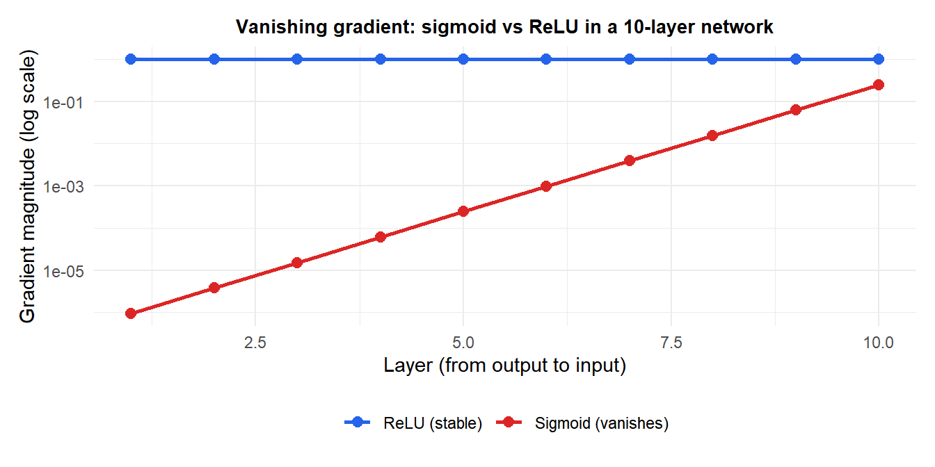
The vanishing gradient problem

In deep networks with sigmoid or tanh activations, the gradient of the loss with respect to early layer weights involves products of many terms like \(\sigma'(z) \leq 0.25\). For a 10-layer network: \(0.25^{10} \approx 10^{-6}\). The gradient effectively vanishes, and early layers learn extremely slowly or not at all.

Regularization

Neural networks have many parameters and overfit easily without regularization.

Dropout

At each training step, randomly set each neuron’s output to zero with probability \(p\) (typically 0.2-0.5). At test time, scale outputs by \((1-p)\). This prevents co-adaptation: no neuron can rely on specific other neurons being present. Equivalent to training an ensemble of \(2^n\) different networks and averaging their predictions.

Batch normalization

After each linear transformation, normalize the activations to zero mean and unit variance across the mini-batch, then scale and shift with learned parameters \(\gamma\) and \(\beta\):

\[\hat{\mathbf{z}} = \frac{\mathbf{z} - \mu_{\mathcal{B}}}{\sqrt{\sigma_{\mathcal{B}}^2 + \varepsilon}}, \qquad \mathbf{a} = \gamma\hat{\mathbf{z}} + \beta\]

Batch norm accelerates training by reducing internal covariate shift, allows higher learning rates, and has a mild regularization effect. It is standard in most modern deep learning architectures.

Weight decay (\(L_2\) regularization)

Add \(\lambda\|\mathbf{W}\|_F^2\) to the loss. Shrinks weights toward zero, reducing model complexity. Equivalent to a Gaussian prior on weights from a Bayesian perspective.

library(torch)

# Define a simple feedforward network
net <- nn_module(
  initialize = function() {
    self$fc1 <- nn_linear(10, 64)
    self$fc2 <- nn_linear(64, 32)
    self$fc3 <- nn_linear(32, 1)
    self$drop <- nn_dropout(p=0.3)
  },
  forward = function(x) {
    x %>% self$fc1() %>% nnf_relu() %>%
          self$drop() %>%
          self$fc2() %>% nnf_relu() %>%
          self$fc3() %>% torch_sigmoid()
  }
)

# With keras (simpler interface)
library(keras)
model <- keras_model_sequential() %>%
  layer_dense(64, activation="relu", input_shape=10) %>%
  layer_batch_normalization() %>%
  layer_dropout(0.3) %>%
  layer_dense(32, activation="relu") %>%
  layer_dense(1,  activation="sigmoid")

model %>% compile(optimizer="adam",
                  loss="binary_crossentropy",
                  metrics="accuracy")
model %>% fit(X_train, y_train, epochs=50,
              batch_size=32, validation_split=0.2)