Naive Bayes
Naive Bayes applies Bayes’ theorem to classification by assuming that all features are conditionally independent given the class label. The assumption is almost always wrong in practice, yet Naive Bayes performs surprisingly well, particularly in text classification where it remains one of the best baselines. Its main advantages are speed, interpretability, and graceful behavior with small training sets.
From Bayes’ theorem to a classifier
The goal is to find the class \(c\) that maximizes the posterior probability given the observed features \(\mathbf{x} = (x_1, \ldots, x_p)\):
\[\hat{c} = \arg\max_c P(C=c \mid \mathbf{x}) = \arg\max_c \frac{P(\mathbf{x} \mid C=c)\, P(C=c)}{P(\mathbf{x})}\]
Since \(P(\mathbf{x})\) is the same for all classes, we only need:
\[\hat{c} = \arg\max_c P(\mathbf{x} \mid C=c)\, P(C=c)\]
The problem: estimating \(P(\mathbf{x} \mid C=c)\) requires the joint distribution of all \(p\) features given the class, which is intractable for large \(p\).
The naive assumption: features are conditionally independent given the class:
\[P(\mathbf{x} \mid C=c) = \prod_{j=1}^p P(x_j \mid C=c)\]
This reduces the estimation to \(p\) univariate problems, one per feature. The classifier becomes:
\[\hat{c} = \arg\max_c P(C=c) \prod_{j=1}^p P(x_j \mid C=c)\]
In practice, products of many small probabilities underflow to zero. Taking logs converts the product to a sum:
\[\hat{c} = \arg\max_c \left[\log P(C=c) + \sum_{j=1}^p \log P(x_j \mid C=c)\right]\]
Three variants
The three variants differ in how they model \(P(x_j \mid C=c)\):
Gaussian Naive Bayes
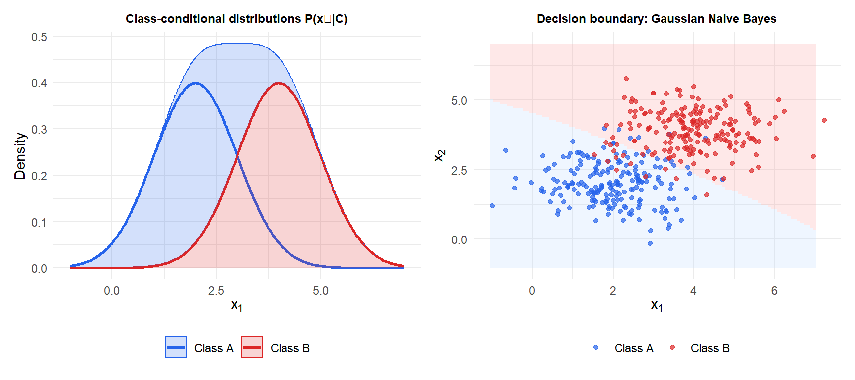
For continuous features, assume each feature follows a Gaussian distribution within each class:
\[P(x_j \mid C=c) = \frac{1}{\sqrt{2\pi\sigma_{jc}^2}} \exp\!\left(-\frac{(x_j - \mu_{jc})^2}{2\sigma_{jc}^2}\right)\]
Parameters \(\mu_{jc}\) and \(\sigma_{jc}^2\) are estimated as the sample mean and variance of feature \(j\) within class \(c\). The decision boundary between two classes is quadratic in general (it becomes linear when \(\sigma_{jc}^2 = \sigma_j^2\) for all \(c\)).
Multinomial Naive Bayes
For count features (e.g., word counts in a document), the likelihood of observing counts \(\mathbf{x} = (x_1, \ldots, x_p)\) given class \(c\) follows a multinomial distribution:
\[P(\mathbf{x} \mid C=c) \propto \prod_{j=1}^p \theta_{jc}^{x_j}\]
where \(\theta_{jc} = P(\text{word } j \mid C=c)\) is estimated as the relative frequency of word \(j\) in class \(c\) documents. This is the standard model for text classification and spam filtering: each email is a bag of words and each word count is a feature.
Bernoulli Naive Bayes
For binary features (word present/absent), each feature follows a Bernoulli distribution:
\[P(x_j \mid C=c) = \theta_{jc}^{x_j}(1-\theta_{jc})^{1-x_j}\]
Unlike Multinomial NB, Bernoulli NB explicitly penalizes the absence of a word: if a word is absent from a document but common in one class, that absence is evidence against that class.
Laplace smoothing
A zero-frequency problem arises in Multinomial and Bernoulli NB: if a word never appears in training documents of class \(c\), then \(\hat{\theta}_{jc} = 0\) and the entire posterior \(P(C=c \mid \mathbf{x}) = 0\) regardless of all other features.
Laplace smoothing (additive smoothing with \(\alpha=1\)) adds a pseudocount of 1 to every feature-class combination:
\[\hat{\theta}_{jc} = \frac{n_{jc} + \alpha}{n_c + \alpha p}\]
where \(n_{jc}\) is the count of feature \(j\) in class \(c\), \(n_c\) is the total count in class \(c\), and \(p\) is the number of features. This ensures no probability is exactly zero while shrinking estimates toward \(1/p\).
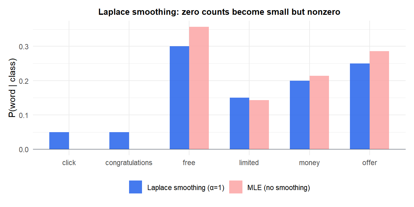
Words “click” and “congratulations” have zero counts under MLE (red), making them catastrophic for any document containing them. Laplace smoothing (blue) assigns them a small but nonzero probability.
Why it works despite wrong assumptions
The independence assumption is almost always violated: words in a sentence are correlated, features in a medical record are correlated, pixel values in an image are correlated. Yet Naive Bayes often performs well. Two explanations:
Classification only needs the right order, not the right probabilities. Even if the estimated probabilities are badly calibrated (and they often are), the ranking of classes by posterior probability may still be correct. Naive Bayes is a poor probability estimator but a good classifier.
Errors cancel. When features are positively correlated within a class, Naive Bayes double-counts their evidence. But it double-counts equally for all classes, so the relative ordering is preserved.
Naive Bayes fails when correlations differ across classes: then the double-counting is unequal and the classifier is biased toward the class with stronger within-class correlations.
Naive Bayes vs logistic regression
Both are linear classifiers (in the log-odds) for binary features. The key difference is the estimation approach:
- Naive Bayes is a generative model: it estimates \(P(\mathbf{x} \mid C=c)\) and \(P(C=c)\) separately, then applies Bayes’ theorem.
- Logistic regression is a discriminative model: it estimates \(P(C \mid \mathbf{x})\) directly.
With Gaussian features and equal covariances, Naive Bayes and LDA produce the same linear boundary. Logistic regression maximizes the conditional likelihood directly and is more efficient asymptotically: it needs less data to match Naive Bayes accuracy when the features are not truly independent.
In practice: Naive Bayes wins with small training sets (less to estimate); logistic regression wins with large training sets (exploits the full data likelihood).
⚠️ Naive Bayes probabilities are poorly calibrated
The posterior probabilities produced by Naive Bayes are often extreme: close to 0 or 1, much more so than the true probabilities. This happens because the independence assumption ignores correlations, causing the model to be overconfident.
If calibrated probabilities are needed (e.g., for decision thresholds in medical diagnosis), apply isotonic regression or Platt scaling after Naive Bayes. Never use Naive Bayes posterior probabilities directly for cost-sensitive decisions without calibration.
💡 Naive Bayes in R
library(e1071)

# Gaussian Naive Bayes (continuous features)
fit_gnb <- naiveBayes(y ~ ., data=df_train)
predict(fit_gnb, newdata=df_test)                    # class labels
predict(fit_gnb, newdata=df_test, type="raw")        # posterior probs

# Laplace smoothing (for categorical/text features)
fit_mnb <- naiveBayes(y ~ ., data=df_train, laplace=1)

# For text classification with a document-term matrix
library(quanteda)
library(quanteda.textmodels)
dtm   <- dfm(corpus)
fit_t <- textmodel_nb(dtm[train_idx,], y[train_idx], smooth=1)
predict(fit_t, newdata=dtm[test_idx,])
