Logistic regression
Logistic regression models the probability of a binary outcome as a function of predictors using the logistic (sigmoid) function. Unlike linear regression, it is estimated by maximum likelihood, not OLS. It is the standard baseline for binary classification and the foundation of neural networks.
The model
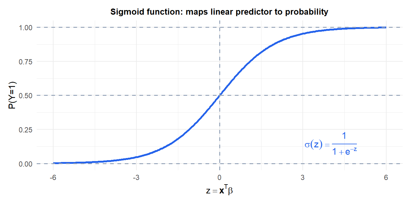
Linear regression applied directly to a binary outcome \(y \in \{0,1\}\) can produce predicted probabilities outside \([0,1]\). Logistic regression fixes this by passing the linear predictor through the sigmoid function:
\[P(Y=1 \mid \mathbf{x}) = \sigma(\mathbf{x}^T\boldsymbol{\beta}) = \frac{1}{1 + e^{-(\beta_0 + \beta_1 x_1 + \cdots + \beta_k x_k)}}\]
The sigmoid maps \((-\infty, +\infty)\) to \((0,1)\) and is S-shaped: it is nearly linear in the middle and saturates at 0 and 1 at the extremes.
Equivalently, the log-odds (logit) of the probability is linear in the predictors:
\[\log\frac{P(Y=1)}{P(Y=0)} = \beta_0 + \beta_1 x_1 + \cdots + \beta_k x_k\]
Maximum likelihood estimation
Since \(y_i \in \{0,1\}\), each observation follows a Bernoulli distribution with \(p_i = \sigma(\mathbf{x}_i^T\boldsymbol{\beta})\). The log-likelihood is:
\[\ell(\boldsymbol{\beta}) = \sum_{i=1}^n \left[y_i \log p_i + (1-y_i)\log(1-p_i)\right]\]
This is the binary cross-entropy (with sign flipped). There is no closed-form solution: \(\nabla \ell = 0\) is solved iteratively by IRLS (Iteratively Reweighted Least Squares) or gradient ascent. Each IRLS step is a weighted OLS problem where the weights are \(w_i = p_i(1-p_i)\) (highest near \(p=0.5\), lowest near 0 or 1).
The Newton-Raphson update:
\[\boldsymbol{\beta}^{(t+1)} = \boldsymbol{\beta}^{(t)} + (\mathbf{X}^T\mathbf{W}^{(t)}\mathbf{X})^{-1}\mathbf{X}^T(\mathbf{y} - \mathbf{p}^{(t)})\]
Interpreting coefficients: odds ratios
A one-unit increase in \(x_j\) multiplies the odds by \(e^{\beta_j}\):
\[\frac{P(Y=1)/(1-P(Y=1))}{P(Y=1|x_j+1)/(1-P(Y=1|x_j+1))} = e^{\beta_j}\]
- \(e^{\beta_j} > 1\): the odds of \(Y=1\) increase with \(x_j\).
- \(e^{\beta_j} < 1\): the odds decrease.
- \(e^{\beta_j} = 1\) (\(\beta_j = 0\)): \(x_j\) has no effect.
Confidence intervals on the odds ratio: \(\left(e^{\hat{\beta}_j - 1.96\cdot\text{SE}},\; e^{\hat{\beta}_j + 1.96\cdot\text{SE}}\right)\).
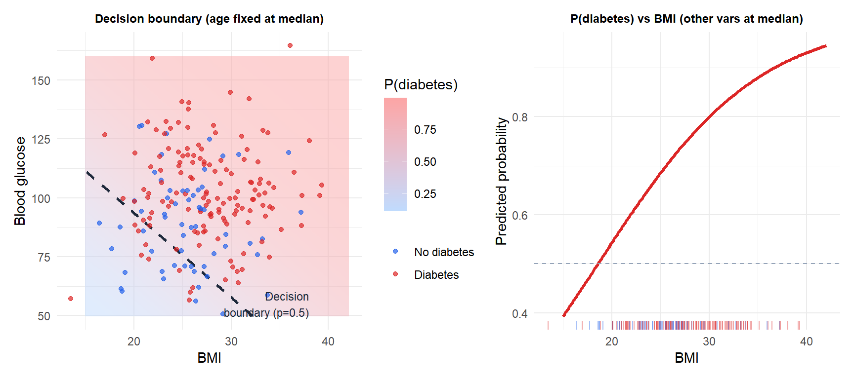
Example: disease risk prediction
Predict whether a patient has diabetes based on age, BMI, and blood glucose level.
Model evaluation
A probability threshold (typically 0.5) converts probabilities to class predictions. The confusion matrix summarizes the results:
| Predicted 0 | Predicted 1 | |
|---|---|---|
| Actual 0 | TN | FP |
| Actual 1 | FN | TP |
Key metrics: accuracy \((TP+TN)/n\), sensitivity/recall \(TP/(TP+FN)\), specificity \(TN/(TN+FP)\), precision \(TP/(TP+FP)\), F1 score.
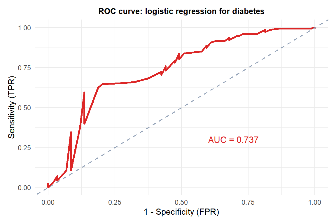
The ROC curve plots sensitivity vs (1-specificity) across all thresholds. The AUC (area under the ROC curve) measures overall discrimination ability: AUC = 0.5 is random; AUC = 1 is perfect.
Extension to multiclass: softmax regression
For \(K > 2\) classes, logistic regression generalizes to softmax (multinomial) regression:
\[P(Y=k \mid \mathbf{x}) = \frac{e^{\mathbf{x}^T\boldsymbol{\beta}_k}}{\sum_{j=1}^K e^{\mathbf{x}^T\boldsymbol{\beta}_j}}\]
Each class \(k\) gets its own coefficient vector \(\boldsymbol{\beta}_k\). The softmax function ensures all \(K\) probabilities sum to 1. One class is taken as the reference (its \(\boldsymbol{\beta}\) is set to zero) for identifiability.
⚠️ Logistic regression fails when classes are perfectly separable
If a linear boundary perfectly separates the two classes (complete separation), the MLE does not exist: the log-likelihood has no maximum, and coefficients diverge to \(\pm\infty\). This is a warning sign that the model is overfit and will generalize poorly.
Symptoms: very large coefficients, enormous standard errors, near-zero predicted probabilities everywhere except at the decision boundary. Solutions: Ridge-penalized logistic regression (glmnet), Firth’s bias-reduced regression (logistf package), or collecting more data.
💡 Logistic regression in R
# Fit logistic regression
fit <- glm(y ~ x1 + x2 + x3, data=df, family=binomial)
summary(fit)
exp(coef(fit))          # odds ratios
exp(confint(fit))       # CI for odds ratios

# Predictions
predict(fit, type="response")   # probabilities
predict(fit, type="link")       # log-odds

# Multinomial logistic regression
library(nnet)
fit_multi <- multinom(y ~ x1 + x2, data=df)

# Ridge-penalized (handles separation)
library(glmnet)
glmnet(X, y, family="binomial", alpha=0)
