K-means clustering
K-means partitions \(n\) observations into \(K\) clusters by minimizing the total within-cluster variance. It alternates between assigning each point to its nearest centroid and recomputing the centroids until convergence. Simple, fast, and scalable to large datasets, K-means is the default starting point for clustering. Its main limitation: it assumes spherical clusters of similar size.
Objective function
K-means minimizes the within-cluster sum of squares (WCSS):
\[\min_{C_1,\ldots,C_K} \sum_{k=1}^K \sum_{\mathbf{x}_i \in C_k} \|\mathbf{x}_i - \boldsymbol{\mu}_k\|^2\]
where \(\boldsymbol{\mu}_k = \frac{1}{|C_k|}\sum_{\mathbf{x}_i \in C_k} \mathbf{x}_i\) is the centroid of cluster \(k\). This is equivalent to maximizing the between-cluster variance: a good clustering concentrates points within clusters and separates clusters from each other.
The optimization is NP-hard in general (exponential number of partitions to check), but the Lloyd’s algorithm finds a local minimum efficiently.
Lloyd’s algorithm
Initialization: place \(K\) centroids in the feature space (see K-means++ below).
Repeat until convergence:
Assignment step: assign each point to its nearest centroid:
\[c_i = \arg\min_{k} \|\mathbf{x}_i - \boldsymbol{\mu}_k\|^2\]
Update step: recompute each centroid as the mean of its assigned points:
\[\boldsymbol{\mu}_k = \frac{1}{|C_k|}\sum_{i: c_i=k} \mathbf{x}_i\]
Each step decreases or maintains the WCSS, so the algorithm always converges. However, it converges to a local minimum, not necessarily the global one.
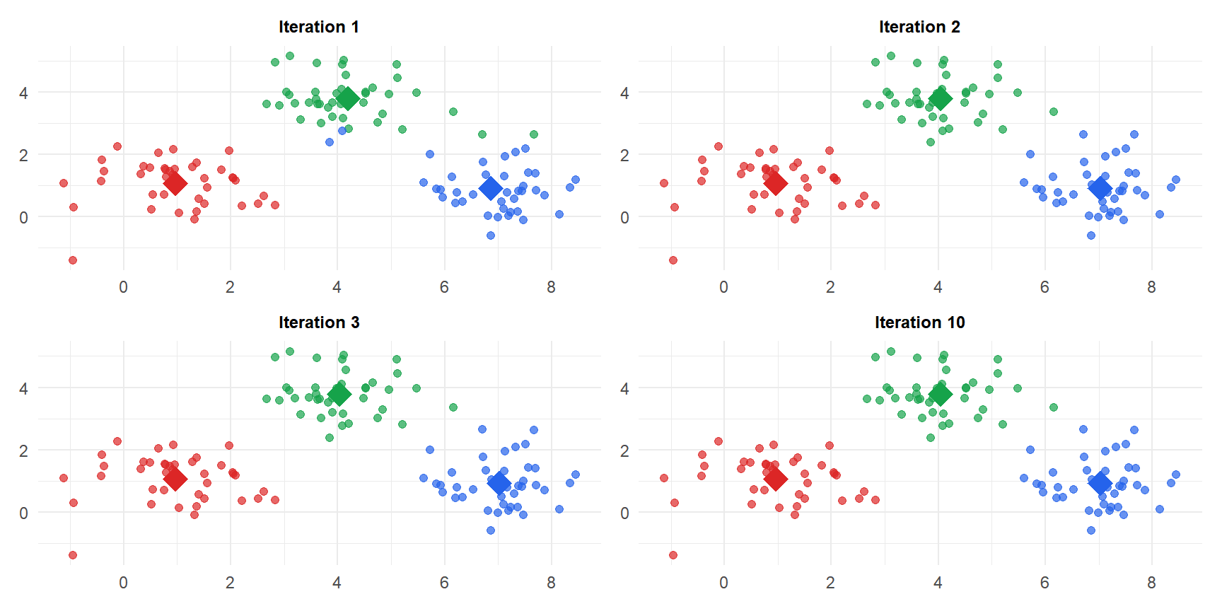
Diamonds are centroids. After iteration 1 the assignments are rough; by iteration 10 the algorithm has converged to the correct three clusters.
K-means++ initialization
Random initialization can lead to poor local minima: if two centroids start in the same cluster, that cluster will be split artificially. K-means++ selects initial centroids that are spread out:
- Choose the first centroid uniformly at random from the data.
- For each subsequent centroid: choose a point with probability proportional to its squared distance from the nearest already-chosen centroid.
- Repeat until \(K\) centroids are chosen.
This gives a \(O(\log K)\) approximation guarantee to the optimal WCSS in expectation, and in practice reduces the number of iterations needed and the probability of poor solutions. K-means++ is the default in most implementations.
Choosing K
Elbow method
Plot WCSS as a function of \(K\). WCSS always decreases as \(K\) increases (with \(K=n\) each point is its own cluster, WCSS=0). The “elbow” is the point where adding another cluster gives diminishing returns.
Silhouette score
For each point \(i\), let \(a_i\) be its mean distance to points in its own cluster and \(b_i\) be its mean distance to points in the nearest other cluster:
\[s_i = \frac{b_i - a_i}{\max(a_i, b_i)} \in [-1, 1]\]
\(s_i \approx 1\): well-clustered. \(s_i \approx 0\): on the boundary between clusters. \(s_i < 0\): probably in the wrong cluster. The mean silhouette score over all points is maximized at the best \(K\).
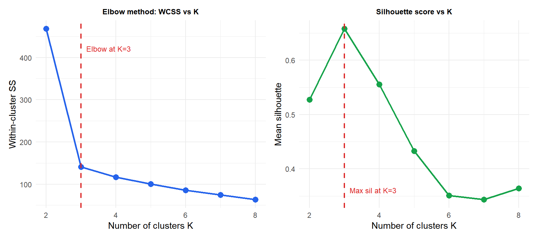
Both methods correctly identify \(K=3\) as optimal for this dataset: the elbow is clear and the silhouette is maximized at \(K=3\).
When K-means fails
K-means assumes clusters are spherical (Euclidean distance to centroid), roughly equal in size, and have similar density. It fails when these assumptions are violated.
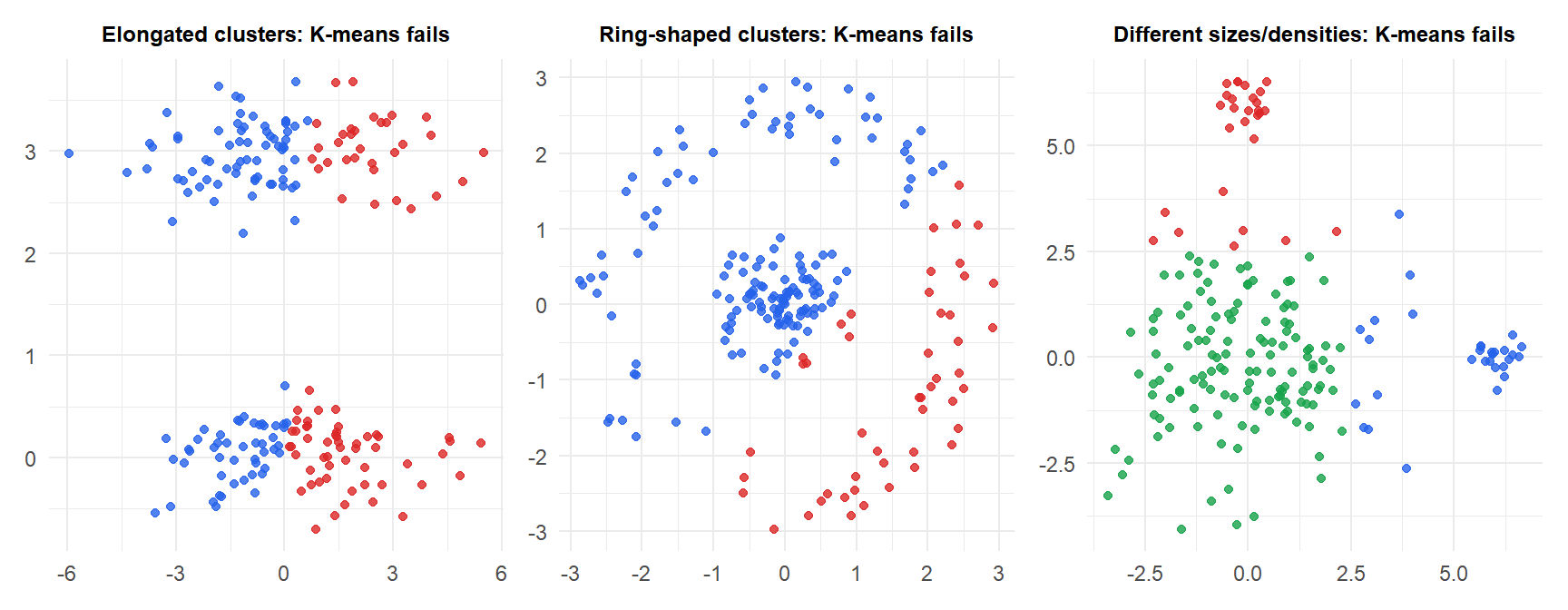
For non-spherical or differently-sized clusters, use DBSCAN (density-based) or hierarchical clustering with appropriate linkage.
⚠️ K-means is sensitive to outliers and feature scale
A single outlier far from any cluster centroid will pull the centroid toward it, distorting the entire cluster. Standardize features before running K-means (otherwise features with large ranges dominate the distance), and consider removing or down-weighting outliers first.
Also: K-means is non-deterministic. Always run with multiple random starts (nstart=20 or more) and take the solution with the lowest WCSS. A single run may converge to a poor local minimum.
💡 K-means in R
# K-means with 20 random starts (best solution returned)
km <- kmeans(X, centers=3, nstart=20, iter.max=100)
km$cluster        # cluster assignments
km$centers        # centroid coordinates
km$tot.withinss   # total WCSS

# Elbow method
wcss <- sapply(1:10, function(k)
  kmeans(X, centers=k, nstart=20)$tot.withinss)
plot(1:10, wcss, type="b", xlab="K", ylab="WCSS")

# Silhouette score
library(cluster)
sil <- silhouette(km$cluster, dist(X))
mean(sil[,3])   # mean silhouette
plot(sil)

# Gap statistic
gap <- clusGap(X, FUN=kmeans, nstart=20, K.max=10, B=50)
plot(gap)
