Gradient boosting and XGBoost
Gradient boosting builds an additive model by sequentially fitting shallow decision trees to the negative gradient of the loss function. Each tree corrects the errors of the current ensemble. XGBoost refines this with second-order Taylor expansion of the loss, explicit regularization on the leaf weights, and a column subsampling that further reduces overfitting. Together they are the dominant algorithm on tabular data competitions.
The core idea: functional gradient descent
Instead of minimizing the loss by updating parameters (as in gradient descent), boosting minimizes the loss by adding functions. The prediction at step \(m\) is:
\[F_m(\mathbf{x}) = F_{m-1}(\mathbf{x}) + \eta \cdot h_m(\mathbf{x})\]
where \(h_m\) is the new tree and \(\eta\) is the learning rate (shrinkage). The tree \(h_m\) is fitted to the negative gradient of the loss evaluated at the current predictions:
\[r_i^{(m)} = -\left[\frac{\partial \mathcal{L}(y_i, F(\mathbf{x}_i))}{\partial F(\mathbf{x}_i)}\right]_{F=F_{m-1}}\]
For squared error loss \(\mathcal{L} = (y_i - F(\mathbf{x}_i))^2/2\): \(r_i^{(m)} = y_i - F_{m-1}(\mathbf{x}_i)\). The trees are fitted to the residuals, which is why early descriptions of boosting talked about “fitting residuals”. The gradient view generalizes this to any differentiable loss: log-loss for classification, absolute error for robust regression, and so on.
The analogy with gradient descent: gradient descent moves in the direction of the negative gradient in parameter space; functional gradient descent moves in the direction of the negative gradient in function space, adding a tree that points in that direction.
The gradient boosting algorithm
- Initialize \(F_0(\mathbf{x}) = \arg\min_\gamma \sum_i \mathcal{L}(y_i, \gamma)\) (e.g., the mean of \(y\) for regression).
- For \(m = 1, \ldots, M\):
- Compute pseudo-residuals \(r_i^{(m)} = -\partial\mathcal{L}/\partial F(\mathbf{x}_i)|_{F_{m-1}}\).
- Fit a shallow tree \(h_m\) to \(\{(\mathbf{x}_i, r_i^{(m)})\}\).
- Update \(F_m = F_{m-1} + \eta \cdot h_m\).
- Return \(F_M\).
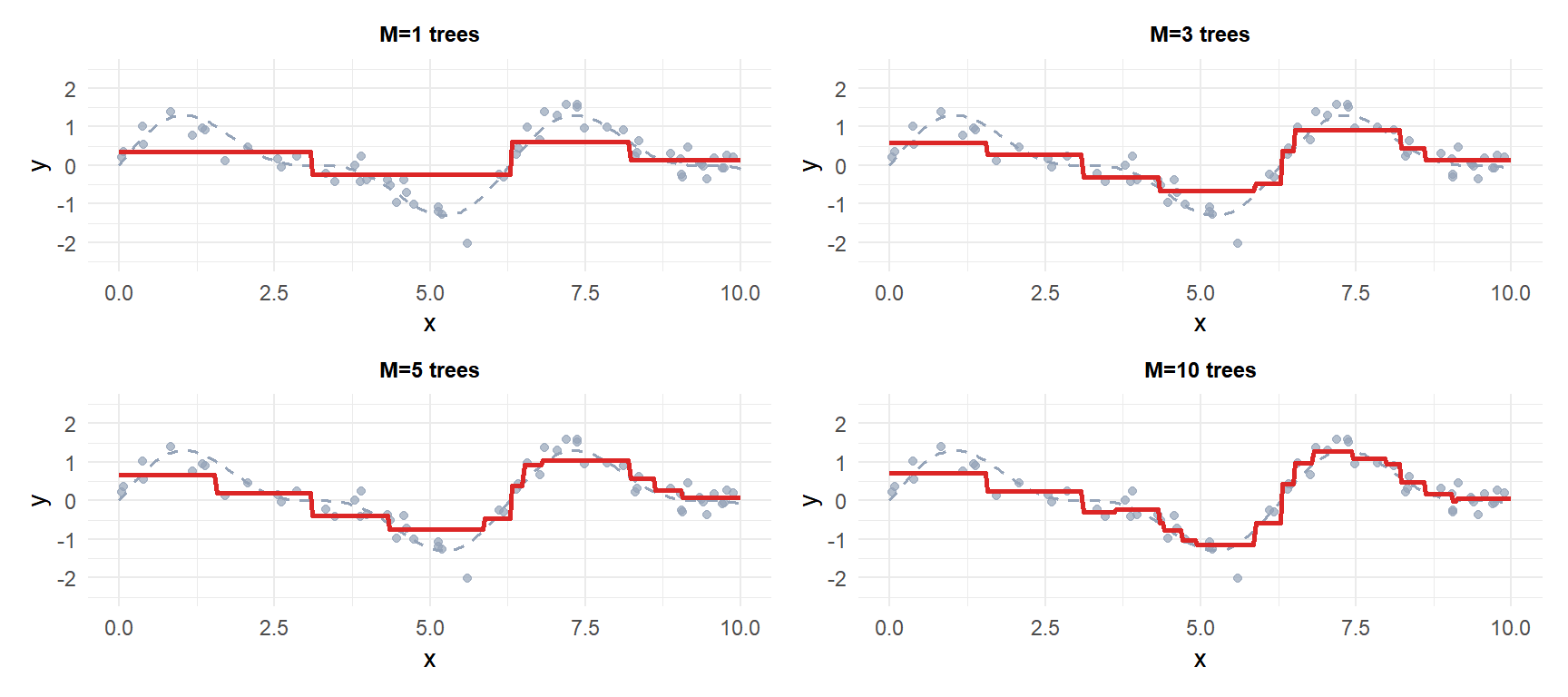
With just 1 tree (top-left) the fit is very rough. As more trees are added the ensemble progressively tracks the true function (grey dashed). The red curve is the current ensemble prediction.
Regularization: the three knobs
Gradient boosting can overfit severely without regularization. Three key controls:
Learning rate \(\eta\) (shrinkage)
Each tree contributes \(\eta \cdot h_m\) instead of \(h_m\). Smaller \(\eta\) requires more trees but produces better generalization. The optimal combination is small \(\eta\) + large \(M\) with early stopping. Typical values: 0.01 to 0.3.
Stochastic gradient boosting (row subsampling)
At each iteration, only a random fraction \(s\) of the training observations (without replacement) is used to fit the tree. This introduces randomness that reduces overfitting and speeds up training. Typical values: \(s = 0.5\) to \(0.8\).
Tree depth
Shallow trees (depth 1-6) are the standard. A depth-1 tree (stump) fits only main effects; depth-2 trees fit pairwise interactions; deeper trees fit higher-order interactions. Boosting typically performs best with shallow trees: most of the complexity comes from combining many trees, not from individual deep ones.
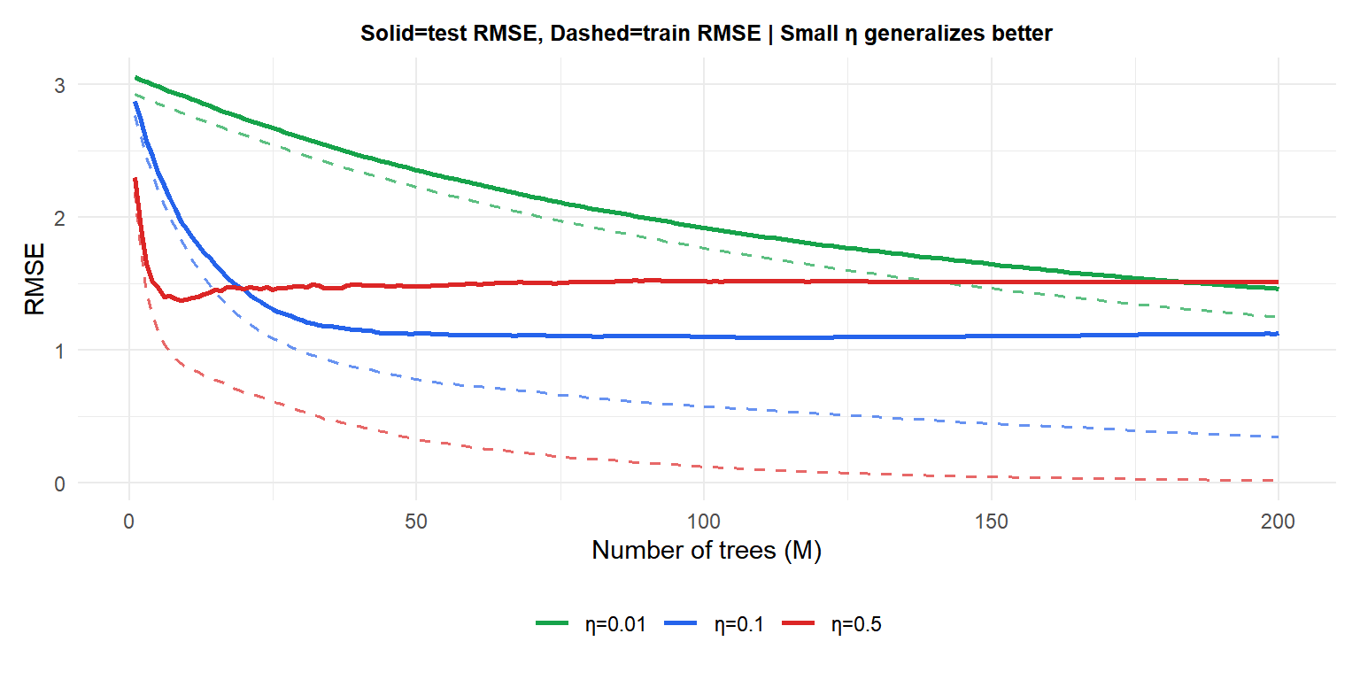
Large \(\eta=0.5\) (red) fits the training data fast but test error rises quickly: overfitting. Small \(\eta=0.01\) (green) descends slowly but reaches a lower test error floor with more trees. Medium \(\eta=0.1\) (blue) balances both.
XGBoost: second-order optimization
Standard gradient boosting uses only the first derivative (gradient) to fit each tree. XGBoost uses a second-order Taylor expansion of the loss:
\[\mathcal{L}^{(m)} \approx \sum_i \left[g_i f_m(\mathbf{x}_i) + \frac{1}{2}h_i f_m(\mathbf{x}_i)^2\right] + \Omega(f_m)\]
where \(g_i = \partial\mathcal{L}/\partial \hat{y}_i\) and \(h_i = \partial^2\mathcal{L}/\partial \hat{y}_i^2\) are the first and second derivatives of the loss at the current prediction, and:
\[\Omega(f_m) = \gamma T + \frac{1}{2}\lambda\sum_{j=1}^T w_j^2\]
penalizes the number of leaves \(T\) and the squared leaf weights \(w_j\) with parameters \(\gamma\) and \(\lambda\).
This formulation gives a closed-form optimal leaf weight for each leaf \(j\):
\[w_j^* = -\frac{\sum_{i \in \text{leaf}_j} g_i}{\sum_{i \in \text{leaf}_j} h_i + \lambda}\]
and an exact gain for each candidate split, making the tree building faster and better calibrated than first-order methods.
Additional XGBoost improvements over classic GBDT:
- Column (feature) subsampling at the tree and split level (like random forest).
- Sparsity-aware split finding: handles missing values and sparse data natively.
- Approximate split finding with quantile sketches: faster than exact search for large \(n\).
- Built-in cross-validation and early stopping.
Random forest vs gradient boosting
| Random forest | Gradient boosting | |
|---|---|---|
| Tree building | Parallel (independent) | Sequential (dependent) |
| Tree depth | Deep (full) | Shallow (depth 3-6) |
| Bias | Low | Decreases with \(M\) |
| Variance | Reduced by averaging | Controlled by \(\eta\), depth, subsampling |
| Overfitting risk | Low (naturally regularized) | High without careful tuning |
| Tuning complexity | Low (mainly mtry) |
Higher (many hyperparameters) |
| Training speed | Fast (parallelizable) | Slower (sequential) |
| Typical accuracy | Very good | Best on tabular data |
Random forest is a safer default: less tuning, harder to overfit. Gradient boosting with XGBoost typically achieves higher accuracy but requires careful hyperparameter selection.
⚠️ Always use early stopping with gradient boosting
Without early stopping, gradient boosting will eventually overfit as \(M\) increases: training error keeps falling while test error rises. Always set aside a validation set or use cross-validation with early stopping:
- Monitor the validation metric at each round.
- Stop when validation error has not improved for \(k\) consecutive rounds (typically \(k=10\) to \(50\)).
- Use the model at the best validation round, not the last one.
With small \(\eta\) (e.g., 0.01), you may need thousands of trees before early stopping triggers: this is expected behavior.
💡 Gradient boosting in R
library(xgboost)

dtrain <- xgb.DMatrix(X_train, label=y_train)
dval   <- xgb.DMatrix(X_val,   label=y_val)

params <- list(
  eta           = 0.05,
  max_depth     = 5,
  subsample     = 0.8,
  colsample_bytree = 0.8,
  lambda        = 1,       # L2 on leaf weights
  gamma         = 0,       # min gain to split
  objective     = "binary:logistic",
  eval_metric   = "auc"
)

fit <- xgb.train(
  params    = params,
  data      = dtrain,
  nrounds   = 1000,
  watchlist = list(train=dtrain, val=dval),
  early_stopping_rounds = 30,
  verbose   = 1
)

# Feature importance
xgb.importance(model=fit)
xgb.plot.importance(xgb.importance(model=fit), top_n=15)

# Cross-validation (no separate val set needed)
cv <- xgb.cv(params=params, data=dtrain, nfold=5,
              nrounds=1000, early_stopping_rounds=30)
best_nrounds <- cv$best_iteration
