Generalized additive model (GAM)
A Generalized Additive Model (GAM) replaces each linear term \(\beta_j x_j\) in a GLM with a smooth function \(f_j(x_j)\). Each smooth is estimated from the data with automatic selection of its complexity. The result is a model that is as flexible as needed for each predictor while remaining interpretable: you can plot and examine the effect of each variable separately.
Formulation
\[g(E[y]) = \beta_0 + f_1(x_1) + f_2(x_2) + \cdots + f_k(x_k)\]
where \(g\) is the link function (identity for Gaussian, logit for binary, log for counts) and each \(f_j\) is a smooth function estimated from the data, typically a penalized regression spline.
The additive structure means the effect of \(x_j\) on \(g(E[y])\) is captured by \(f_j\) while holding all other predictors constant, just as in linear regression. The difference: \(f_j\) can be any smooth curve, not just a line.
Non-linear interactions between two predictors can be included with tensor product smooths: \(f(x_1, x_2)\), a smooth surface over two variables.
Automatic smoothness selection: REML
Each smooth \(f_j\) is estimated by minimizing a penalized criterion:
\[\text{Penalized deviance} = -2\ell(\boldsymbol{\beta}) + \sum_j \lambda_j \int [f_j''(x)]^2 dx\]
The penalty \(\lambda_j\) controls the wiggliness of \(f_j\). Too small: overfits. Too large: degenerates to a straight line. The mgcv package selects all \(\lambda_j\) automatically by REML (Restricted Maximum Likelihood), which gives better variance estimation than GCV for most practical cases.
The complexity of each smooth is summarized by its effective degrees of freedom (edf):
- edf = 1: the smooth has been penalized to a straight line.
- edf = 2: approximately quadratic.
- edf close to \(k\) (the maximum): very wiggly, little penalization.
Large edf means strong nonlinearity; edf near 1 means the predictor could be included linearly.
Example: air quality modeling
Model daily ozone concentration as a function of solar radiation, wind speed, and temperature. A linear model assumes constant rates of change; a GAM allows each relationship to be nonlinear.
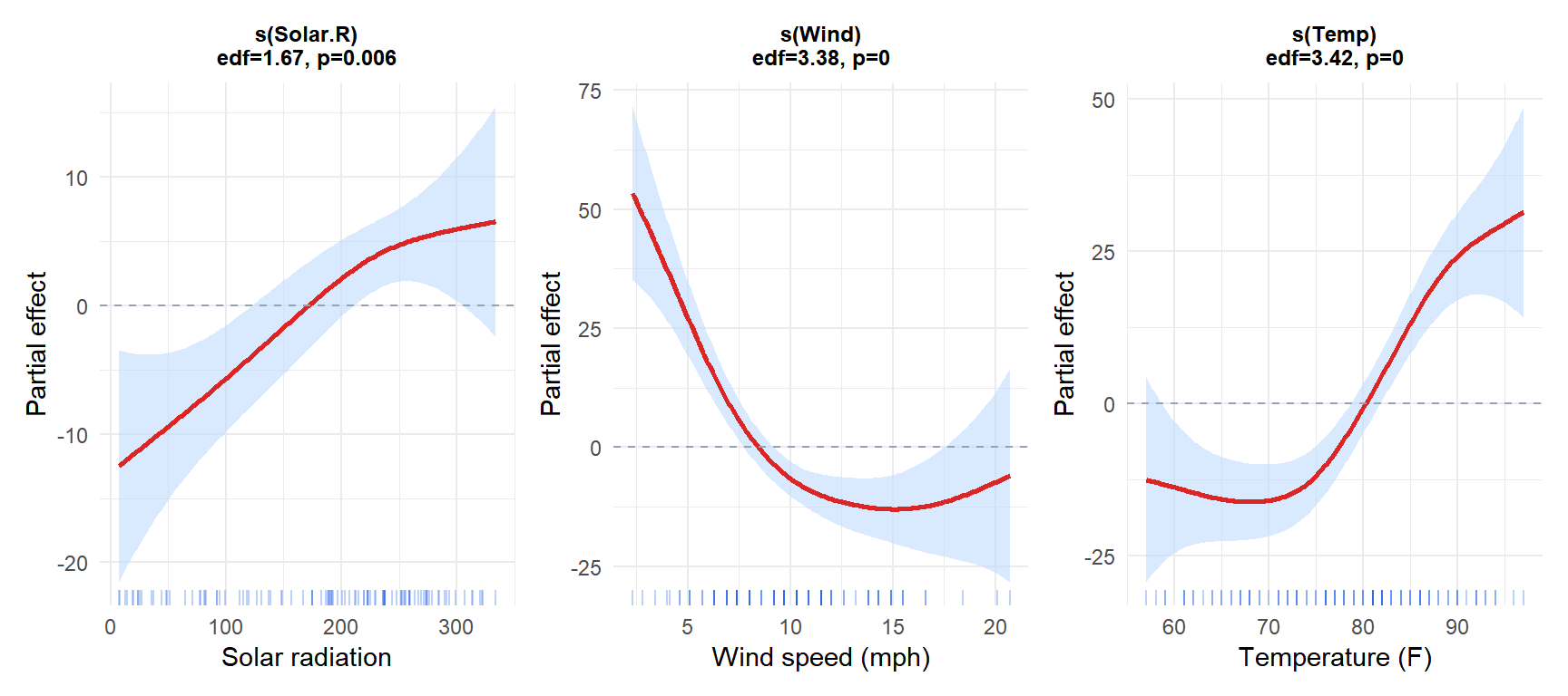
Each panel shows the partial effect of one predictor: how much it contributes to the predicted ozone after accounting for the other two. The shaded band is the 95% pointwise confidence interval. The rug shows the data density.
Temperature has a strongly nonlinear positive effect (edf >> 1). Wind has a monotone negative effect, nearly linear. Solar radiation has a moderate positive effect with some curvature.
GAM vs linear model: when does it matter?
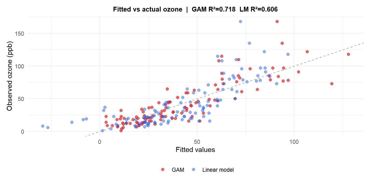
The GAM fits the data substantially better than the linear model (\(R^2\) is higher) because it captures the nonlinear effects of temperature and wind on ozone concentration.
Model diagnostics
After fitting, check:
- Residuals vs fitted: should show no pattern (same as linear regression).
gam.check(): plots four diagnostic panels and tests whether the basis dimension \(k\) is large enough for each smooth. If the \(p\)-value from the \(k\)-index test is significant, increase \(k\).concurvity(): the GAM equivalent of multicollinearity. Measures how much one smooth can be approximated by a combination of other smooths. High concurvity inflates standard errors.
⚠️ Smooth terms can absorb each other if predictors are correlated
If two predictors are strongly correlated (e.g., temperature and month), their smooth terms compete to explain the same variation. The individual smooth plots may look flat or implausible even if the overall model fits well. Check concurvity(fit) and consider whether both smooths are scientifically justified or whether one should be dropped or replaced by a tensor product interaction.
Extensions
GAMs generalize naturally:
- GAMM (GAM with random effects): adds random effects for grouped data. Fitted with
gamm()orgamm4. - Non-Gaussian responses: binary (
family=binomial), counts (family=poisson), survival data. - Tensor product smooths:
te(x1, x2)for nonlinear interactions between two continuous predictors. - Factor smooths:
s(x, by=group)fits a separate smooth for each level of a factor, allowing the shape of the relationship to differ by group.
💡 GAMs in R with mgcv
library(mgcv)

# Gaussian GAM (default)
fit <- gam(y ~ s(x1) + s(x2) + x3, data=df, method="REML")
summary(fit)   # edf, p-values for each smooth, R², deviance explained

# Binary outcome
fit_bin <- gam(y ~ s(x1) + s(x2), data=df,
               family=binomial, method="REML")

# Count data
fit_pois <- gam(count ~ s(x), family=poisson, method="REML", data=df)

# Diagnostics
gam.check(fit)       # residual plots + basis dimension test
concurvity(fit)      # correlation between smooths
plot(fit, pages=1)   # all smooth term plots

# Tensor product interaction
fit_te <- gam(y ~ te(x1, x2), data=df, method="REML")
