Decision trees
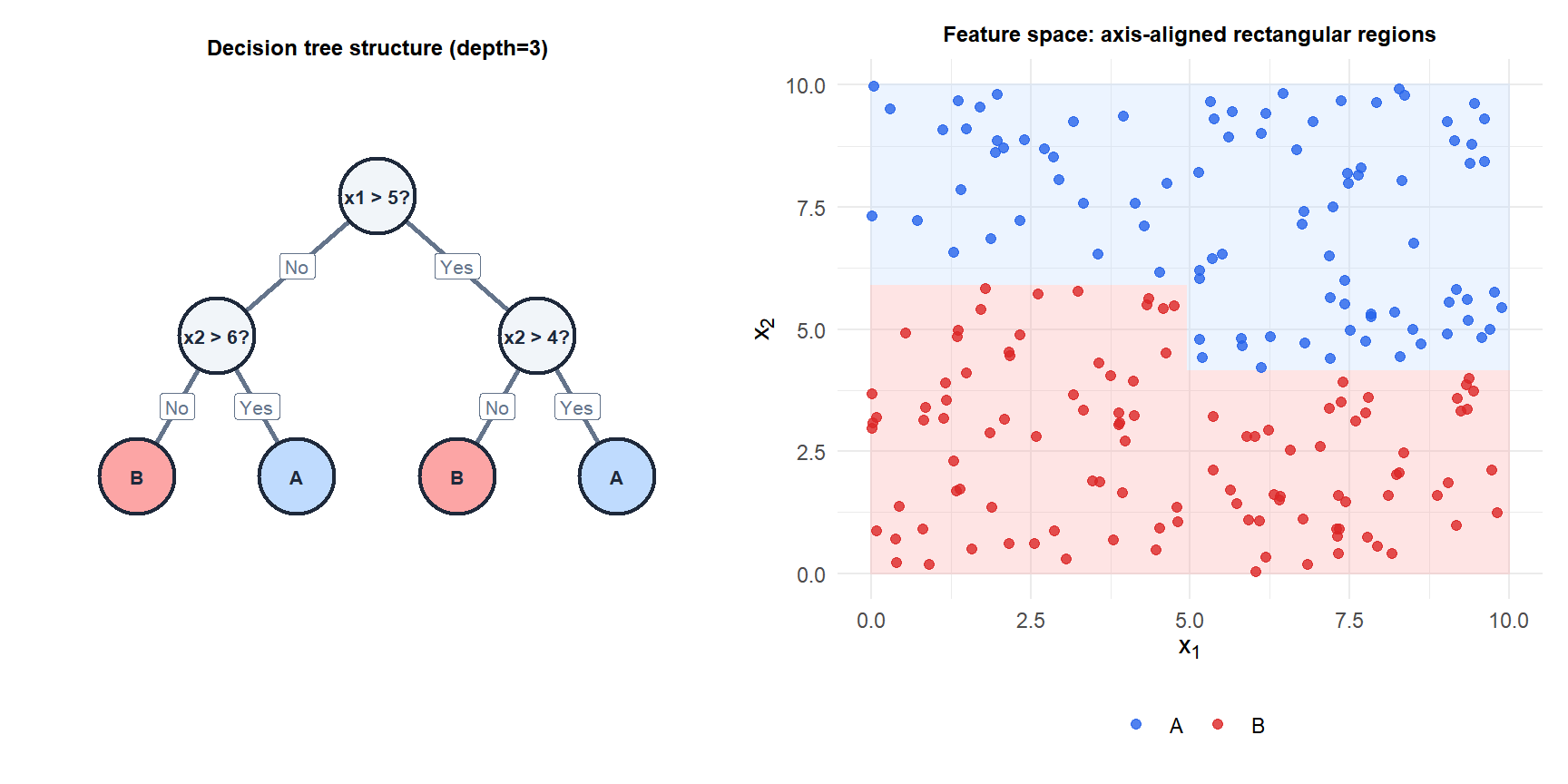
A decision tree partitions the feature space into rectangular regions by recursively splitting on the feature and threshold that best separates the classes (or reduces prediction error for regression). The result is an interpretable, axis-aligned partition: every prediction is a sequence of yes/no questions about the features. Trees are the building block of the most powerful ensemble methods: random forests and gradient boosting.
Recursive binary partitioning
The CART (Classification and Regression Trees) algorithm builds a tree top-down:
- At each node, consider every feature \(j\) and every possible split threshold \(t\).
- Choose the \((j, t)\) pair that minimizes the weighted impurity of the two resulting child nodes.
- Recurse on each child until a stopping criterion is met (maximum depth, minimum node size, or no improvement possible).
- Assign each leaf node the majority class (classification) or mean response (regression).
The split search is greedy: at each node, the locally best split is chosen without looking ahead. This does not guarantee a globally optimal tree, but the problem of finding the globally optimal tree is NP-hard.
Split criteria: measuring impurity
For a node containing \(n\) points of which \(n_k\) belong to class \(k\), with \(\hat{p}_k = n_k/n\):
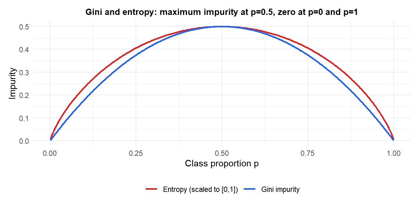
Gini impurity
\[G = \sum_{k=1}^K \hat{p}_k(1-\hat{p}_k) = 1 - \sum_{k=1}^K \hat{p}_k^2\]
Measures the probability of misclassifying a randomly chosen point using the node’s class distribution. \(G=0\) for a pure node (one class), \(G=0.5\) for maximum impurity in a binary problem. Default in CART.
Information gain (entropy)
\[H = -\sum_{k=1}^K \hat{p}_k \log_2 \hat{p}_k\]
Information gain at a split = entropy of parent minus weighted entropy of children. Tends to prefer splits that produce more balanced children than Gini, but results are usually similar in practice.
MSE (regression trees)
\[\text{MSE} = \frac{1}{n}\sum_{i \in \text{node}} (y_i - \bar{y}_\text{node})^2\]
The best split minimizes the weighted sum of MSE in the two child nodes.
Pruning: preventing overfitting
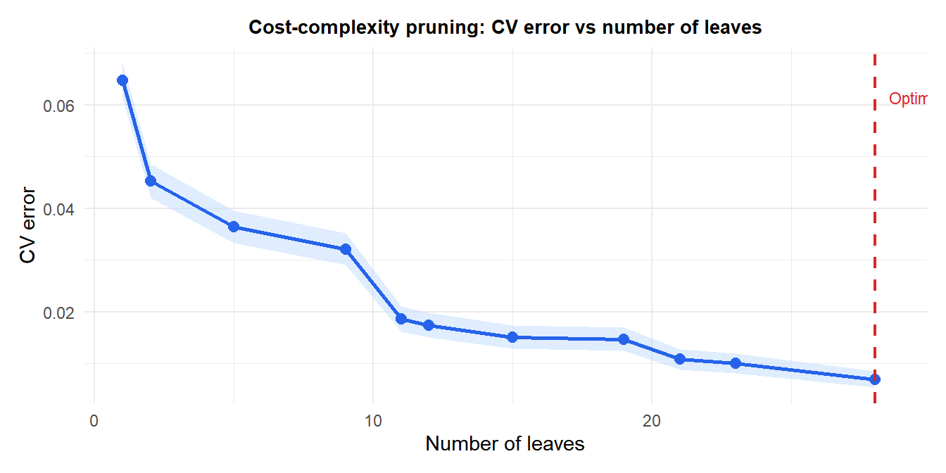
A fully grown tree (no stopping criterion) perfectly fits the training data but generalizes poorly: it memorizes noise. Cost-complexity pruning (weakest-link pruning) controls this by adding a penalty for tree size:
\[R_\alpha(T) = R(T) + \alpha|T|\]
where \(R(T)\) is the training misclassification rate, \(|T|\) is the number of leaves, and \(\alpha \geq 0\) is the complexity parameter. For each \(\alpha\), there is a unique subtree \(T_\alpha\) that minimizes \(R_\alpha\). As \(\alpha\) increases, branches are progressively pruned until only the root remains.
The optimal \(\alpha\) is selected by cross-validation: fit the full tree, generate the sequence of subtrees for increasing \(\alpha\), and choose the \(\alpha\) that minimizes CV error.
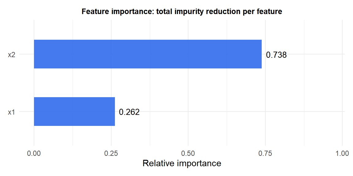
Feature importance
The importance of feature \(j\) is the total reduction in impurity achieved by all splits on \(j\), weighted by the number of samples reaching each split:
\[\text{Importance}(j) = \sum_{\text{splits on } j} \frac{n_\text{node}}{n} \cdot \Delta\text{Impurity}\]
Features used near the root (where more samples pass through) contribute more. This gives an interpretable ranking of feature relevance, though it can be biased toward features with more unique values.
Properties of decision trees
Advantages:
- Interpretable: can be visualized and explained to non-technical audiences.
- No feature scaling required: splits are threshold comparisons, not distances.
- Handles mixed feature types: numerical and categorical natively.
- Automatically captures interactions between features.
- Robust to outliers in the response (outliers only affect one leaf).
Limitations:
- High variance: small changes in the training data can produce completely different trees. A single data point near a split threshold can change the entire tree structure below that split.
- Axis-aligned boundaries: cannot capture diagonal decision boundaries without many splits.
- Biased toward features with many unique values.
- Suboptimal: the greedy split strategy does not find the globally best tree.
⚠️ Single decision trees are rarely competitive
The high variance of individual trees makes them poor predictors on their own. They are almost always used as building blocks for ensemble methods:
- Bagging and random forests: average many deep trees trained on bootstrap samples, reducing variance while preserving low bias.
- Gradient boosting: build shallow trees sequentially, each correcting the errors of the previous ones.
A single pruned decision tree is valuable for interpretability and as a baseline, but if prediction accuracy is the goal, always compare against random forest or gradient boosting before settling on a single tree.
💡 Decision trees in R
library(rpart)

# Fit a classification tree
fit <- rpart(y ~ ., data=df_train, method="class",
             control=rpart.control(cp=0))   # grow full tree

# Visualize
library(rpart.plot)
rpart.plot(fit, type=4, extra=101)

# Cost-complexity pruning: choose cp by CV
printcp(fit)
plotcp(fit)

# Prune to optimal cp (1-SE rule)
best_cp <- fit$cptable[which.min(fit$cptable[,"xerror"]), "CP"]
fit_pruned <- prune(fit, cp=best_cp)

# Feature importance
fit$variable.importance / sum(fit$variable.importance)

# Regression tree
fit_reg <- rpart(y ~ ., data=df_train, method="anova")
