DBSCAN
DBSCAN (Density-Based Spatial Clustering of Applications with Noise) defines clusters as dense regions of points separated by sparse regions. It requires no \(K\) upfront, detects outliers automatically as noise points, and finds clusters of arbitrary shape. Its two parameters, \(\varepsilon\) and minPts, define what counts as “dense”.
Core concepts: density and reachability
\(\varepsilon\)-neighborhood of a point \(p\): the set of all points within distance \(\varepsilon\) from \(p\):
\[N_\varepsilon(p) = \{q \in D : d(p,q) \leq \varepsilon\}\]
Point types (relative to parameters \(\varepsilon\) and minPts):
- Core point: \(|N_\varepsilon(p)| \geq \text{minPts}\). Has enough neighbors to define a dense region.
- Border point: \(|N_\varepsilon(p)| < \text{minPts}\) but \(p \in N_\varepsilon(q)\) for some core point \(q\). On the edge of a cluster.
- Noise point (outlier): neither core nor border. Isolated from any dense region.
Density-reachability: point \(q\) is density-reachable from core point \(p\) if there is a chain of core points \(p = p_1, p_2, \ldots, p_k = q\) where each \(p_{i+1} \in N_\varepsilon(p_i)\).
A cluster is a maximal set of density-connected points: every point in the cluster is density-reachable from every core point in the cluster.
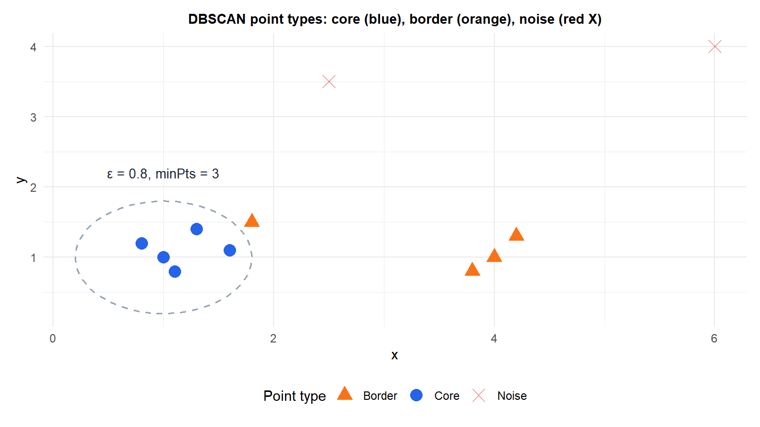
The dashed circles show the \(\varepsilon\)-neighborhood of two core points. Blue core points have at least minPts neighbors within \(\varepsilon\); orange border points are within \(\varepsilon\) of a core but do not meet minPts themselves; the red X is noise.
The algorithm
For each unvisited point p:
  Mark p as visited
  If |N_eps(p)| < minPts:
    Label p as Noise
  Else:
    Create a new cluster C
    Add p to C
    Add all points in N_eps(p) to a seed set S
    For each point q in S:
      If q is unvisited:
        Mark q as visited
        If |N_eps(q)| >= minPts:
          Add N_eps(q) to S
      If q is not yet in a cluster:
        Add q to C
With a spatial index (kd-tree or ball tree), the complexity is \(O(n \log n)\). Without one (brute force): \(O(n^2)\). The algorithm is deterministic given \(\varepsilon\) and minPts: no random initialization.
DBSCAN vs K-means on non-spherical data
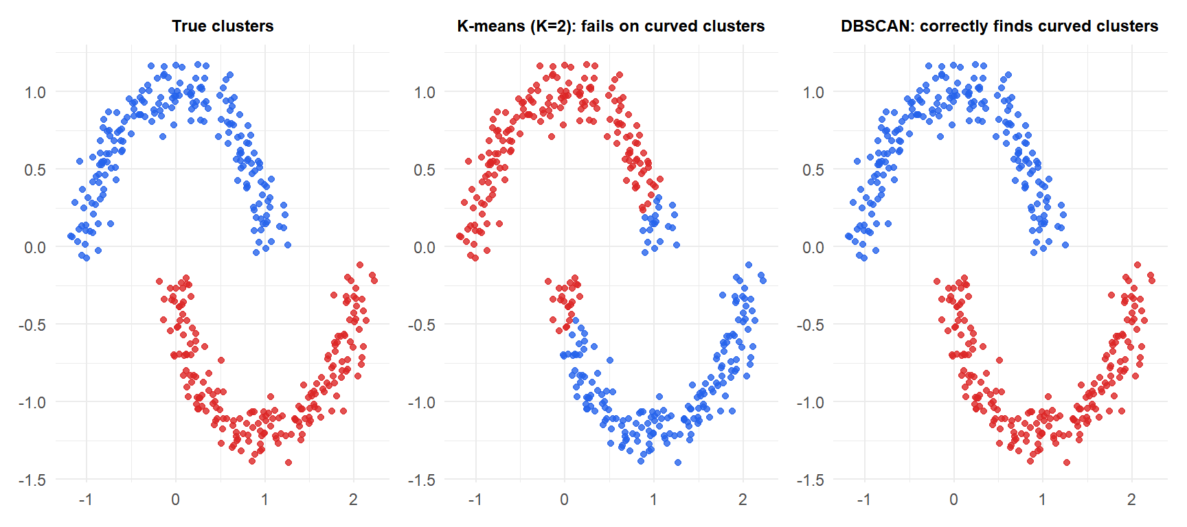
K-means forces a Voronoi partition: it draws a straight boundary between the two moons and misclassifies half of each. DBSCAN follows the density of each moon and correctly recovers both curved clusters.
Choosing \(\varepsilon\) and minPts
minPts
A common rule of thumb: minPts \(\geq\) dimensionality + 1, typically set to 4 or 5 for 2D data, and increasing with dimensionality. Higher minPts makes the algorithm more robust to noise but may miss small clusters.
\(\varepsilon\): the k-distance plot
For each point, compute the distance to its \(k\)-th nearest neighbor (\(k\) = minPts - 1). Sort these distances in descending order and plot them. The “elbow” of this k-distance plot suggests a good \(\varepsilon\): below the elbow, most points are core; above it, most are noise.
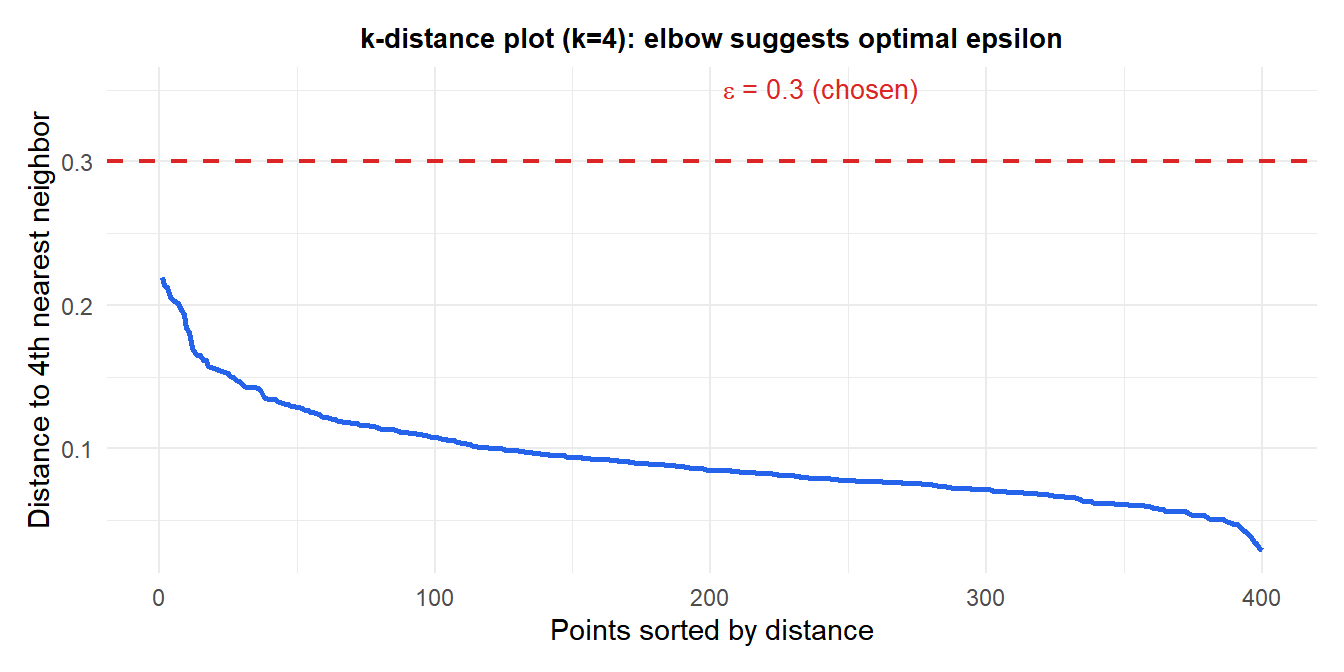
The steep drop in the sorted k-distances marks the boundary between core and noise points. The red dashed line at \(\varepsilon=0.3\) is where the elbow occurs.
When DBSCAN fails
DBSCAN assumes clusters have uniform density. It struggles when:
- Clusters of varying density: a single \(\varepsilon\) may be too small for sparse clusters (they fragment into noise) and too large for dense ones (they merge). HDBSCAN (hierarchical DBSCAN) addresses this by building a hierarchy of density levels.
- High dimensions: the curse of dimensionality makes all points roughly equidistant, so no single \(\varepsilon\) separates dense from sparse regions. DBSCAN loses its meaning beyond \(d \approx 10\)-15 features.
- Very large datasets: even with spatial indexing, \(\varepsilon\)-neighborhood queries can be slow in high dimensions.
⚠️ DBSCAN cluster labels are not stable across runs with different parameters
DBSCAN is deterministic given \(\varepsilon\) and minPts, but the cluster labels (which cluster gets label 1, 2, etc.) can differ between implementations or runs on reordered data. Border points that fall within \(\varepsilon\) of multiple clusters are assigned to whichever core point is processed first.
More importantly: small changes in \(\varepsilon\) can cause large changes in the clustering. Always try a range of \(\varepsilon\) values near the k-distance elbow and check that results are stable. A result that changes completely with a 10% change in \(\varepsilon\) is not trustworthy.
💡 DBSCAN in R
library(dbscan)

# k-distance plot to choose epsilon
kNNdistplot(X, k=4)
abline(h=0.3, col="red", lty=2)

# Fit DBSCAN
db <- dbscan(X, eps=0.3, minPts=5)
db$cluster   # 0 = noise, 1,2,... = clusters
table(db$cluster)

# Plot results
plot(X, col=db$cluster+1, pch=20)

# HDBSCAN (handles varying density)
hdb <- hdbscan(X, minPts=5)
plot(hdb$hc)   # dendrogram of condensed cluster tree

# LOF (Local Outlier Factor): continuous density-based anomaly score
lof_scores <- lof(X, minPts=5)
plot(X, col=ifelse(lof_scores > 2, "red","black"), pch=20)
