Bias-variance tradeoff
The bias-variance tradeoff is the central tension in supervised machine learning. Every prediction error can be decomposed into three components: bias (systematic error from wrong assumptions), variance (sensitivity to training data fluctuations), and irreducible noise. Reducing bias tends to increase variance and vice versa. Understanding this tradeoff guides every decision about model complexity, regularization, and data collection.
The bias-variance decomposition
Let \(y = f(x) + \varepsilon\) where \(f\) is the true function and \(\varepsilon \sim (0, \sigma^2)\) is irreducible noise. For a model \(\hat{f}\) trained on dataset \(\mathcal{D}\), the expected prediction error at a point \(x\) is:
\[E\left[(y - \hat{f}(x))^2\right] = \underbrace{\left[f(x) - E[\hat{f}(x)]\right]^2}_{\text{Bias}^2} + \underbrace{E\left[\left(\hat{f}(x) - E[\hat{f}(x)]\right)^2\right]}_{\text{Variance}} + \underbrace{\sigma^2}_{\text{Irreducible noise}}\]
The expectation is taken over all possible training datasets \(\mathcal{D}\) of the same size:
- Bias: how far the average prediction is from the true value. Error from wrong assumptions baked into the model (e.g., fitting a line to nonlinear data).
- Variance: how much the prediction fluctuates across different training sets. A model with high variance memorizes the training data and fails to generalize.
- Irreducible noise \(\sigma^2\): the inherent randomness in \(y\) that no model can remove. A lower bound on prediction error regardless of model complexity.
The total expected error is the sum of all three. Bias and variance cannot both be minimized simultaneously with a fixed amount of data: this is the tradeoff.
Intuition: the target analogy
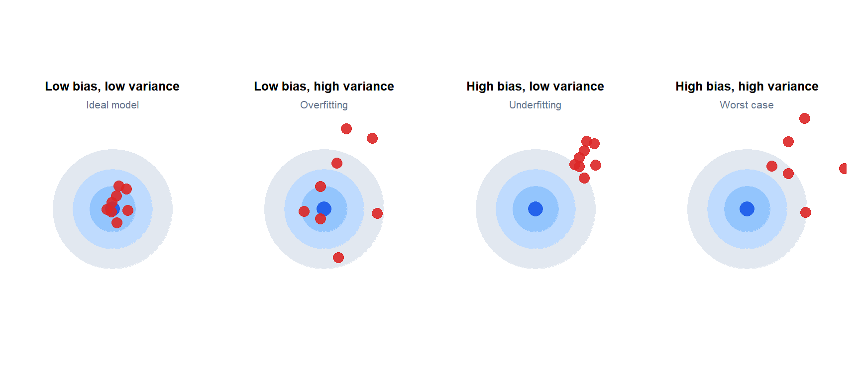
Shots on a target: each shot is a prediction from a model trained on a different dataset. Low bias means shots are centered on the bullseye. Low variance means shots are tightly clustered. The ideal model (top-left) achieves both.
Model complexity and the tradeoff
As model complexity increases (more parameters, higher polynomial degree, fewer regularization constraints):
- Bias decreases: the model is flexible enough to capture the true pattern.
- Variance increases: the model is sensitive to the specific training set and fits noise.
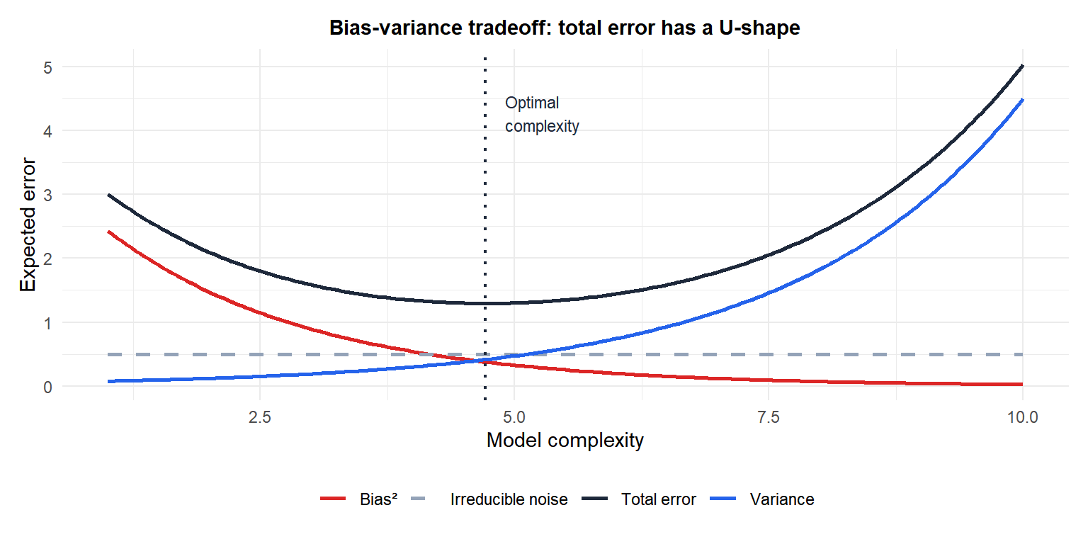
Total error (black) has a U-shape. The optimal complexity minimizes the sum of bias and variance. Too simple (left): high bias dominates. Too complex (right): high variance dominates. The irreducible noise (grey dashed) sets the floor.
Concrete example: polynomial regression
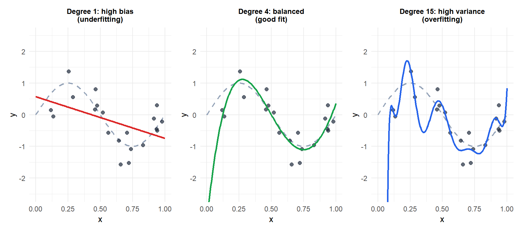
Grey dashed: true function \(\sin(2\pi x)\). Black dots: training data with noise. Red (degree 1) misses the pattern: high bias. Green (degree 4) approximates the true function well. Blue (degree 15) passes through every training point but oscillates wildly: high variance.
Managing the tradeoff in practice
Several strategies directly address the bias-variance tradeoff:
Reducing variance (at some cost to bias):
- Regularization (Ridge, Lasso): penalizes model complexity, shrinking coefficients toward zero. Increases bias slightly, reduces variance substantially.
- Ensemble methods (random forests, bagging): average predictions from many high-variance models to reduce variance without increasing bias.
- More training data: variance decreases as \(O(1/n)\); bias is unaffected. The most reliable fix when data is available.
- Dropout (neural networks): randomly deactivates neurons during training, acting as an implicit ensemble.
Reducing bias (at some cost to variance):
- More complex models: more parameters, higher-degree polynomials, deeper networks.
- Feature engineering: adding relevant features that the model was missing.
- Boosting: sequentially build models that correct the bias of previous ones (XGBoost, AdaBoost).
⚠️ Cross-validation estimates total error, not bias and variance separately
Test error (estimated via cross-validation) is the sum of bias, variance and noise. A model with low test error could achieve it through low bias, low variance, or both. You cannot directly observe the individual components from test error alone.
To empirically decompose bias and variance, you need multiple training sets from the same distribution: train the model on each, compute predictions at the same test points, then estimate bias as the squared difference between average prediction and truth, and variance as the spread of predictions across training sets. In practice this is rarely feasible; the decomposition is mostly a theoretical guide.
💡 The bias-variance tradeoff and model selection
Use the following mental model when choosing between models:
- High training error, high test error: high bias. The model is too simple. Try more complexity, more features, or a different model class.
- Low training error, high test error: high variance. The model overfits. Try regularization, more data, or a simpler model.
- Both errors are similar and acceptable: the model generalizes well. The tradeoff is well-managed.
The gap between training and test error is a direct proxy for variance. The level of training error is a proxy for bias (relative to the irreducible noise floor).

