Types of Errors in Statistics
Every hypothesis test can make two types of mistakes: rejecting a true null hypothesis (Type I error) or failing to reject a false one (Type II error). Understanding these errors, their probabilities, and the tradeoff between them is essential for designing and interpreting statistical tests correctly.
Definition
When we make a decision in a hypothesis test, we are comparing our conclusion against the unknown truth. Four outcomes are possible:
| \(H_0\) is true | \(H_0\) is false | |
|---|---|---|
| Reject \(H_0\) | Type I error (\(\alpha\)) | Correct decision (power \(= 1-\beta\)) |
| Fail to reject \(H_0\) | Correct decision | Type II error (\(\beta\)) |
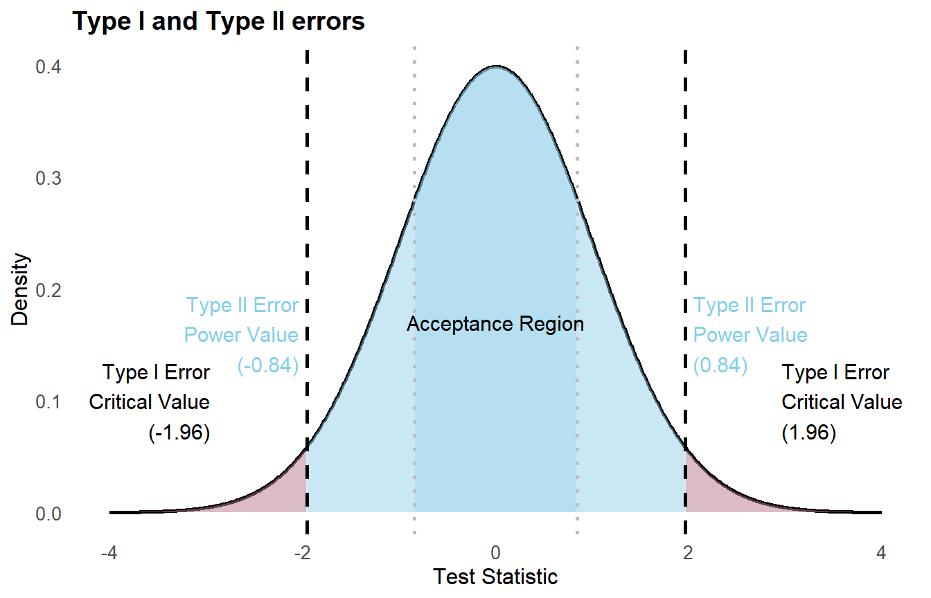
- Type I Error (False Positive)
A Type I error occurs when \(H_0\) is rejected even though it is true. The probability of this error is \(\alpha\), the significance level. By setting \(\alpha = 0.05\), we accept a 5% chance of incorrectly rejecting a true null hypothesis.
- Type II Error (False Negative)
A Type II error occurs when we fail to reject \(H_0\) even though it is false. Its probability is \(\beta\). The power of the test is \(1 - \beta\): the probability of correctly detecting a real effect. A common target is power \(= 0.80\).
Real-world examples
- Medical diagnosis
\(H_0\): the patient does not have the disease. \(H_1\): the patient has the disease.
- Type I error: the test says the patient has the disease when they do not (false positive). Consequence: unnecessary anxiety, further testing, or harmful treatment.
- Type II error: the test says the patient is healthy when they actually have the disease (false negative). Consequence: delayed treatment, disease progression.
In screening programs for serious diseases, minimizing Type II errors is often prioritized: missing a real case can be life-threatening, while a false positive leads only to a confirmatory test.
- Quality control
\(H_0\): the production batch meets quality standards. \(H_1\): the batch is defective.
- Type I error: rejecting a good batch (false alarm). Consequence: unnecessary waste and production cost.
- Type II error: accepting a defective batch. Consequence: defective products reach customers.
The balance between the two costs depends on the product. For safety-critical components (aircraft parts, medical devices), minimizing Type II errors justifies higher Type I error rates.
- Legal system
\(H_0\): the defendant is innocent. \(H_1\): the defendant is guilty.
- Type I error: convicting an innocent person. “Beyond reasonable doubt” sets \(\alpha\) very low.
- Type II error: acquitting a guilty person.
Most legal systems deliberately accept higher Type II error rates to minimize wrongful convictions.
The tradeoff and how to manage it
For fixed sample size, reducing \(\alpha\) increases \(\beta\) (and reduces power). The only way to reduce both simultaneously is to increase \(n\).
The power of a test depends on four factors:
- \(\alpha\): larger \(\alpha\) increases power but also Type I error risk.
- \(n\): larger samples always increase power.
- Effect size \(\delta\): larger true differences are easier to detect.
- \(\sigma\): less variable populations give higher power.
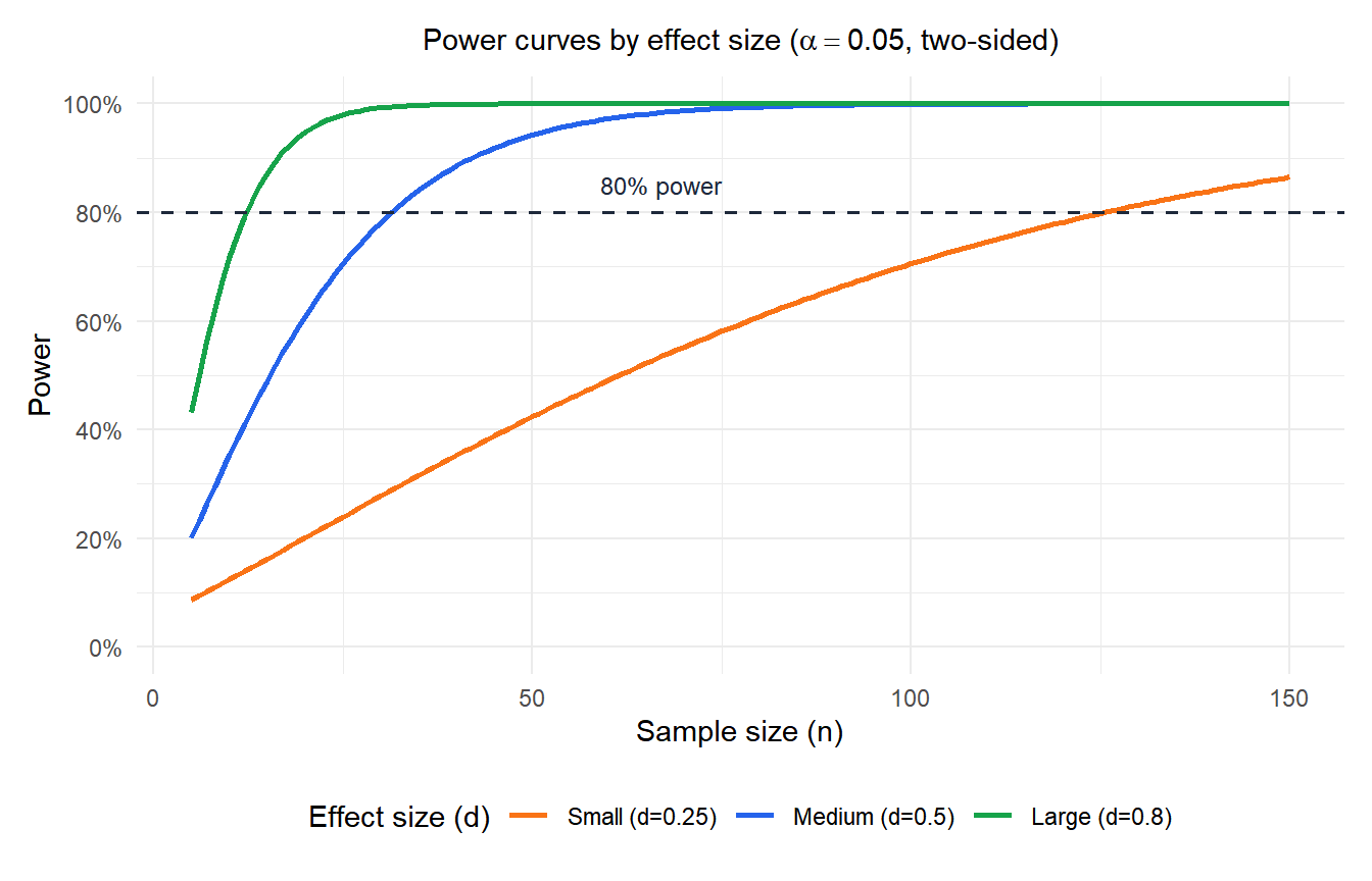
For small effects (\(d = 0.25\)), achieving 80% power requires 125 observations. For medium effects (\(d = 0.5\)), around 35 suffice. For large effects (\(d = 0.8\)), fewer than 15 are enough. This is why underpowered studies with small samples often fail to detect real effects.
⚠️ Underpowered studies: a systemic problem
Many published studies are underpowered: they use sample sizes too small to reliably detect the effects they claim to study. An underpowered study that finds a significant result may be detecting a spuriously large effect (due to sampling variability), while one that finds no significance may simply have been unable to detect a real but small effect.
Always compute power before collecting data. A study with power below 0.50 is unlikely to be informative regardless of its result.
💡 Practical guidelines for managing errors
- Set \(\alpha\) before collecting data, based on the cost of a Type I error in your context.
- Target power \(\geq 0.80\) (80%), ideally 0.90 for confirmatory studies.
- Use power analysis to determine \(n\) before starting data collection.
- When the cost of a Type II error is high (medical screening, safety testing), use higher \(\alpha\) or larger \(n\) to boost power.
- Report both \(\alpha\) and the achieved power so readers can assess the reliability of your conclusions.

