Two-sample z-test for proportions
The two-sample z-test for proportions evaluates whether two population proportions are equal. Under \(H_0: p_1 = p_2\), both groups share the same proportion, so a pooled estimate is used to compute the standard error. This is what distinguishes the test from the confidence interval for \(p_1 - p_2\), which uses individual estimates.
Hypotheses
| Test | \(H_0\) | \(H_1\) |
|---|---|---|
| Two-sided | \(p_1 = p_2\) | \(p_1 \neq p_2\) |
| One-sided right | \(p_1 = p_2\) | \(p_1 > p_2\) |
| One-sided left | \(p_1 = p_2\) | \(p_1 < p_2\) |
Test statistic
Given \(x_1\) successes in \(n_1\) trials and \(x_2\) successes in \(n_2\) trials:
\[\hat{p}_1 = \frac{x_1}{n_1}, \quad \hat{p}_2 = \frac{x_2}{n_2}\]
Under \(H_0\), both groups share a common proportion \(p\). It is estimated by pooling:
\[\hat{p} = \frac{x_1 + x_2}{n_1 + n_2}\]
The test statistic is:
\[Z = \frac{\hat{p}_1 - \hat{p}_2}{\sqrt{\hat{p}(1-\hat{p})\left(\dfrac{1}{n_1} + \dfrac{1}{n_2}\right)}}\]
Under \(H_0\) and the normal approximation, \(Z \sim N(0,1)\).
⚠️ Pooled SE for the test, unpooled SE for the confidence interval
The test statistic uses the pooled proportion \(\hat{p}\) in the standard error, because under \(H_0\) the two groups have the same true proportion and pooling gives a better estimate of it.
The confidence interval for \(p_1 - p_2\) uses the unpooled standard error \(\sqrt{\hat{p}_1(1-\hat{p}_1)/n_1 + \hat{p}_2(1-\hat{p}_2)/n_2}\), because the CI does not assume \(H_0\) is true.
Using the unpooled SE in the test (or the pooled SE in the CI) is incorrect.
The normal approximation is valid when all four counts are at least 10:
\[n_1\hat{p} \geq 10, \quad n_1(1-\hat{p}) \geq 10, \quad n_2\hat{p} \geq 10, \quad n_2(1-\hat{p}) \geq 10\]
For small counts, use Fisher’s exact test.
Examples
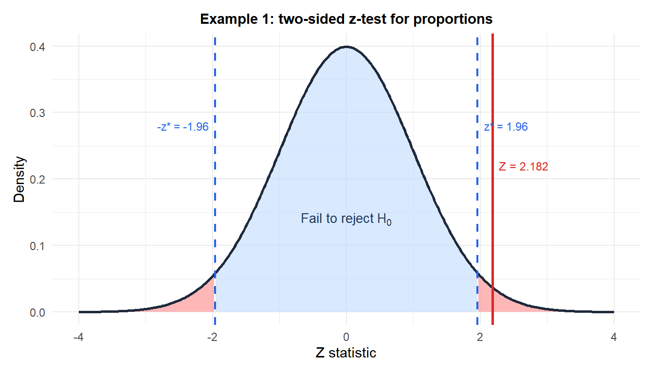
Example 1: conversion rate A/B test (two-sided)
An e-commerce platform tests two checkout page designs. Version A: 180 purchases out of 600 visitors (\(\hat{p}_1 = 0.300\)). Version B: 156 purchases out of 600 visitors (\(\hat{p}_2 = 0.260\)). Is there a significant difference in conversion rate?
Pooled proportion:
\[\hat{p} = \frac{180 + 156}{600 + 600} = \frac{336}{1200} = 0.280\]
Check conditions: \(600 \times 0.280 = 168 \geq 10\), \(600 \times 0.720 = 432 \geq 10\). Valid.
Test statistic:
\[Z = \frac{0.300 - 0.260}{\sqrt{0.280 \times 0.720 \times (1/600 + 1/600)}} = \frac{0.040}{\sqrt{0.2016/600}} = \frac{0.040}{0.01833} \approx 2.182\]
p-value (two-sided): \(p = 2 \times P(Z \geq 2.182) \approx 0.029\).
Decision: \(p = 0.029 < 0.05\), reject \(H_0\). Version A has a significantly higher conversion rate.
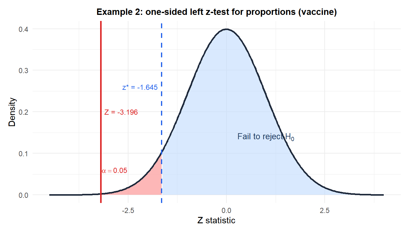
Example 2: vaccine efficacy (one-sided right)
A clinical trial assigns 500 participants to vaccine and 500 to placebo. Infections: 18 in the vaccine group (\(\hat{p}_1 = 0.036\)) and 42 in the placebo group (\(\hat{p}_2 = 0.084\)). Is the vaccine effective (lower infection rate)?
Hypotheses: \(H_0: p_1 = p_2\) vs \(H_1: p_1 < p_2\) (one-sided left, vaccine has lower rate).
Pooled proportion:
\[\hat{p} = \frac{18 + 42}{1000} = 0.060\]
Test statistic:
\[Z = \frac{0.036 - 0.084}{\sqrt{0.060 \times 0.940 \times (1/500 + 1/500)}} = \frac{-0.048}{\sqrt{0.0002256}} = \frac{-0.048}{0.01502} \approx -3.196\]
p-value (one-sided left): \(p = P(Z \leq -3.196) \approx 0.001\).
Decision: \(p = 0.001 < 0.05\), reject \(H_0\). The vaccine significantly reduces the infection rate.
Connection with the chi-squared test
For a \(2 \times 2\) contingency table, the two-sided z-test for proportions and the chi-squared test of independence are mathematically equivalent: \(Z^2 = \chi^2\) with \(df = 1\). For Example 1: \(Z^2 = 2.182^2 = 4.761 \approx \chi^2_{(1)}\).
The chi-squared test generalizes to tables larger than \(2 \times 2\); the z-test is specific to two proportions and also handles one-sided alternatives, which the chi-squared test does not.
Running the test in R
prop.test() in R performs this test using the chi-squared approximation (equivalent to the z-test for two proportions):
# Example 1: A/B test (two-sided)
prop.test(x = c(180, 156), n = c(600, 600),
          alternative = "two.sided", correct = FALSE)

# Example 2: vaccine (one-sided left)
prop.test(x = c(18, 42), n = c(500, 500),
          alternative = "less", correct = FALSE)

# Fisher's exact test for small counts
fisher.test(matrix(c(18, 482, 42, 458), nrow = 2))
correct = FALSE disables the Yates continuity correction. The correction is conservative and generally not recommended for large samples.
💡 Reporting the result
Report the two proportions, their difference, and its confidence interval alongside the test result. For Example 1: “Version A converted at 30.0% vs 26.0% for Version B, a difference of 4.0 percentage points (95% CI: 0.5% to 7.5%; \(Z = 2.18\), \(p = 0.029\)).” The CI tells you the range of plausible effect sizes, which the p-value alone does not.

