Sign test
The sign test is the simplest nonparametric test. It only uses the direction of each observation relative to a reference value (positive or negative), ignoring magnitudes entirely. This makes it extremely robust but also less powerful than alternatives that use more of the data.
How it works
Given \(n\) observations (or differences), record the sign of each one relative to the hypothesized median \(M_0\):
- \(+\) if the observation is above \(M_0\).
- \(-\) if the observation is below \(M_0\).
- Ties (exact equality to \(M_0\)) are discarded.
Under \(H_0\) (the true median is \(M_0\)), each non-tied observation is equally likely to be positive or negative, so the number of positive signs \(S^+\) follows a \(\text{Binomial}(n, 0.5)\) distribution.
| Test | \(H_0\) | \(H_1\) | p-value |
|---|---|---|---|
| Two-sided | \(M = M_0\) | \(M \neq M_0\) | \(2 \times P(X \leq \min(S^+, S^-))\) |
| One-sided right | \(M = M_0\) | \(M > M_0\) | \(P(X \geq S^+)\) |
| One-sided left | \(M = M_0\) | \(M < M_0\) | \(P(X \leq S^+)\) |
where \(X \sim \text{Binomial}(n, 0.5)\) and \(n\) is the number of non-tied observations.
Examples
Example 1: paired data (teaching method)
Ten students take a test before and after a new teaching intervention. Score differences (after - before):
\[+3,\; +1,\; -2,\; +4,\; +2,\; 0,\; -1,\; +3,\; +1,\; -2\]
Step 1: discard the zero difference. \(n = 9\).
Step 2: count signs. \(S^+ = 6\) (positive), \(S^- = 3\) (negative).
Step 3: two-sided p-value from \(X \sim \text{Binomial}(9, 0.5)\):
\[p = 2 \times P(X \leq 3) = 2 \times \sum_{k=0}^{3} \binom{9}{k} 0.5^9 = 2 \times 0.254 = 0.508\]
Decision: \(p = 0.508 > 0.05\), fail to reject \(H_0\).
No significant evidence that the teaching method changed the median score. The 6-3 split in signs is not unusual under \(H_0\).
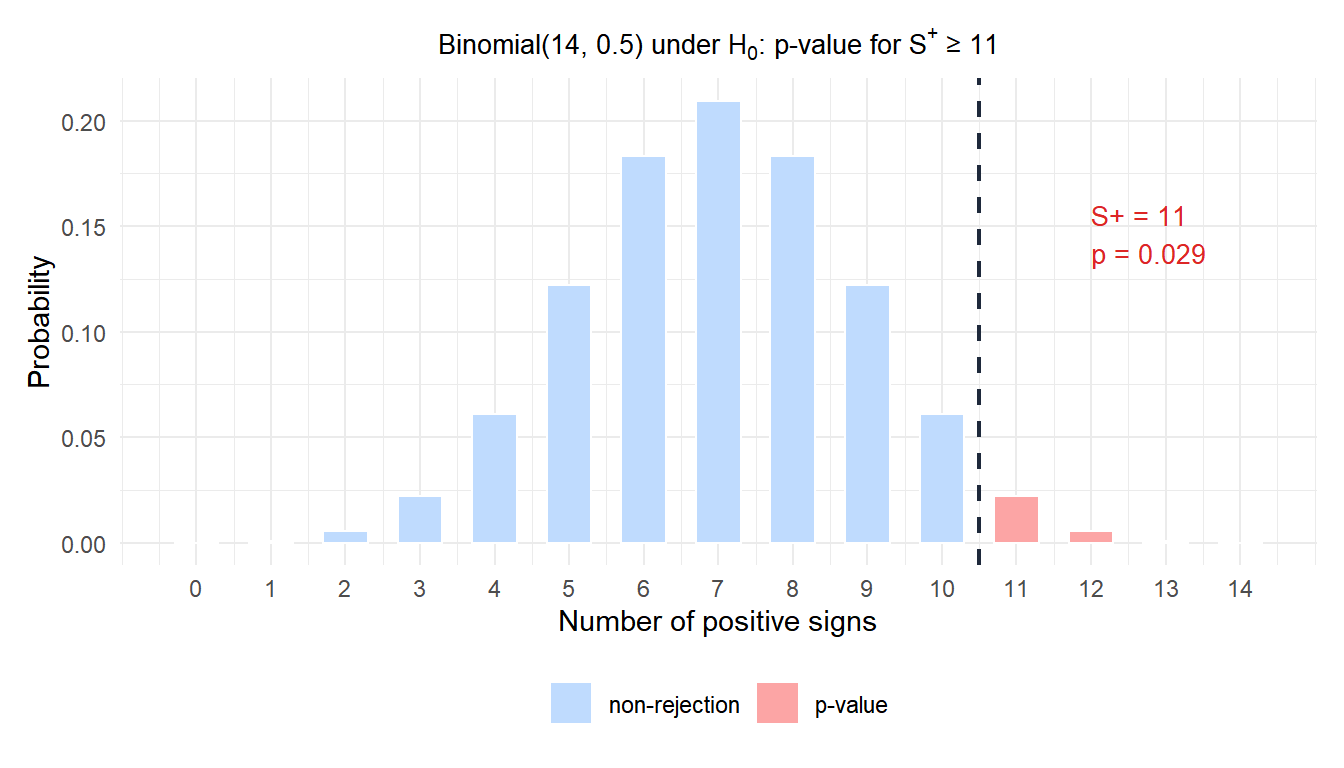
Example 2: one-sample test for the median
A delivery service claims their median delivery time is 48 hours. A consumer group records 15 deliveries: 11 took more than 48 hours, 3 took less, and 1 took exactly 48 hours.
Step 1: discard the tie. \(n = 14\), \(S^+ = 11\), \(S^- = 3\).
Step 2: one-sided right test (\(H_1: M > 48\)). P-value:
\[p = P(X \geq 11) = \sum_{k=11}^{14} \binom{14}{k} 0.5^{14} = 0.029\]
Decision: \(p = 0.029 < 0.05\), reject \(H_0\).
There is significant evidence that the true median delivery time exceeds 48 hours.
Sign test vs Wilcoxon signed-rank test
Both are nonparametric alternatives to the paired \(t\)-test, but they use different amounts of information:
| Sign test | Wilcoxon signed-rank | |
|---|---|---|
| Uses direction | Yes | Yes |
| Uses magnitude | No | Yes (via ranks) |
| Assumes symmetric differences | No | Yes |
| Power | Lower | Higher |
| Best for | Ordinal data, outliers, heavy skew | Continuous, roughly symmetric differences |
⚠️ Use Wilcoxon signed-rank when you can
The sign test discards all information about magnitude, which costs power. For the same data, the Wilcoxon signed-rank test is almost always more powerful because it ranks the absolute differences and considers their relative sizes.
Use the sign test when:
- The data are ordinal and differences have no meaningful magnitude (e.g., ranked preferences).
- The differences are so heavily skewed or have such extreme outliers that even ranks are unreliable.
- You need the absolute minimum of assumptions.
In most situations with continuous paired data, the Wilcoxon signed-rank test is the better choice.
Running the test in R
There is no dedicated sign.test() in base R. The easiest approach uses the binomial test directly:
# Example 2: delivery times
# S+ = 11 successes out of n = 14 non-tied observations
binom.test(x = 11, n = 14, p = 0.5, alternative = "greater")

# For paired data: compute differences first
diffs <- c(3, 1, -2, 4, 2, -1, 3, 1, -2)  # excluding the zero
s_plus <- sum(diffs > 0)
n      <- sum(diffs != 0)
binom.test(s_plus, n, p = 0.5, alternative = "two.sided")

# The BSDA package also provides sign.test()
library(BSDA)
sign.test(diffs, md = 0, alternative = "two.sided")
💡 Large sample approximation
For \(n > 25\), the binomial distribution under \(H_0\) is well-approximated by a normal distribution:
\[Z = \frac{S^+ - n/2}{\sqrt{n/4}} \sim N(0,1)\]
This is useful for quick hand calculations. For exact p-values with any \(n\), use the binomial directly as shown above.

