Shapiro-Wilk test
The Shapiro-Wilk test is the most powerful test for normality for small to medium samples. It compares the observed order statistics to what a normal distribution would predict, and summarizes the agreement in a single statistic \(W\) between 0 and 1.
Hypotheses
\(H_0\): the data come from a normally distributed population.
\(H_1\): the data do not come from a normally distributed population.
Reject \(H_0\) when \(p \leq \alpha\). Failing to reject \(H_0\) does not prove normality: it means the data are consistent with normality at the chosen significance level.
The W statistic
The test statistic is:
\[W = \frac{\left(\sum_{i=1}^{n} a_i x_{(i)}\right)^2}{\sum_{i=1}^{n}(x_i - \bar{x})^2}\]
where \(x_{(i)}\) are the ordered sample values and \(a_i\) are coefficients derived from the expected values of order statistics of a standard normal distribution. The denominator is proportional to the sample variance.
\(W\) ranges between 0 and 1. A value close to 1 means the observed quantiles match normal quantiles well. Small values of \(W\) indicate departures from normality.
The p-value is obtained by comparing \(W\) to its exact distribution (computed by Shapiro and Wilk via simulation), not from a standard table.
Examples
Example 1: normally distributed data
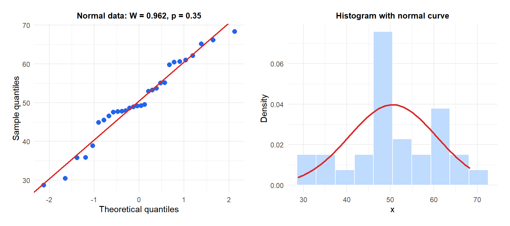
Points follow the diagonal closely and \(W \approx 1\): no evidence against normality.
Example 2: right-skewed data
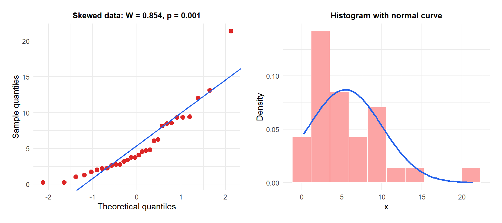
Points curve away from the diagonal in the upper tail (right skew). \(W\) is substantially below 1 and \(p < 0.05\): normality is rejected.
Interpreting W and the p-value
A useful way to read the result:
- \(W > 0.95\) and \(p > 0.05\): strong consistency with normality.
- \(W\) between 0.90 and 0.95 and \(p > 0.05\): mild departure, likely not problematic for robust parametric tests.
- \(W < 0.90\) or \(p \leq 0.05\): meaningful departure from normality. Inspect the Q-Q plot to understand the nature of the departure (skewness, heavy tails, outliers).
The Q-Q plot always provides more information than the p-value alone: it shows where the data depart from normality, not just whether they do.
⚠️ Large samples: the test becomes too sensitive
For \(n > 100\), Shapiro-Wilk detects trivial departures from normality that have no practical consequence for parametric tests. A dataset with \(n = 500\) might give \(W = 0.993\) and \(p = 0.012\), rejecting normality despite the data being essentially normal for any practical purpose.
For large samples, rely on the Q-Q plot and consider the robustness of your downstream test. The \(t\)-test and ANOVA are quite robust to mild non-normality when \(n\) is large, thanks to the CLT.
⚠️ Small samples: the test has low power
For \(n < 15\), Shapiro-Wilk rarely rejects \(H_0\) even for clearly non-normal data. A non-significant result with small samples is weak evidence of normality. Again, the Q-Q plot is essential.
Running the test in R
The test is built into base R and requires no packages:
shapiro.test(x)The output gives \(W\) and the p-value. For a complete normality assessment, complement with a Q-Q plot:
qqnorm(x)
qqline(x)
The Shapiro-Wilk test in R is limited to samples between 3 and 5,000 observations. For \(n > 5,000\), use the Anderson-Darling test from the nortest package: nortest::ad.test(x).
💡 When normality is rejected: what to do next
Rejecting \(H_0\) does not automatically mean parametric tests are invalid. Consider:
- The downstream test’s robustness: \(t\)-tests and ANOVA are fairly robust to mild non-normality for \(n \geq 30\).
- Transformations: log, square root, or Box-Cox transformations often normalize right-skewed data.
- Non-parametric alternatives: Wilcoxon signed-rank instead of one-sample \(t\), Mann-Whitney instead of two-sample \(t\), Kruskal-Wallis instead of ANOVA.
- Bootstrap methods: resample-based confidence intervals and tests require no normality assumption.
The goal is not to achieve a non-significant Shapiro-Wilk result but to use a method appropriate for the actual distribution of your data.

