Power of a test

The power of a test is the probability of correctly rejecting a false null hypothesis. A test with low power misses real effects: it produces many false negatives. Planning for adequate power before collecting data is one of the most important steps in study design.

Definition

Power is defined as:

where \(\beta = P(\text{fail to reject } H_0 \mid H_1 \text{ is true})\) is the Type II error probability. A power of 0.80 means there is an 80% chance of detecting a real effect if one exists.

Power depends on four quantities, all interconnected:

• Effect size \(\delta\): how large the true difference is.
• Sample size \(n\): more data always increases power.
• Significance level \(\alpha\): larger \(\alpha\) increases power but also Type I error risk.
• Population variability \(\sigma\): less variable populations are easier to study.

If you fix three of these, the fourth is determined. Power analysis uses this relationship to find the minimum \(n\) needed to achieve a target power.

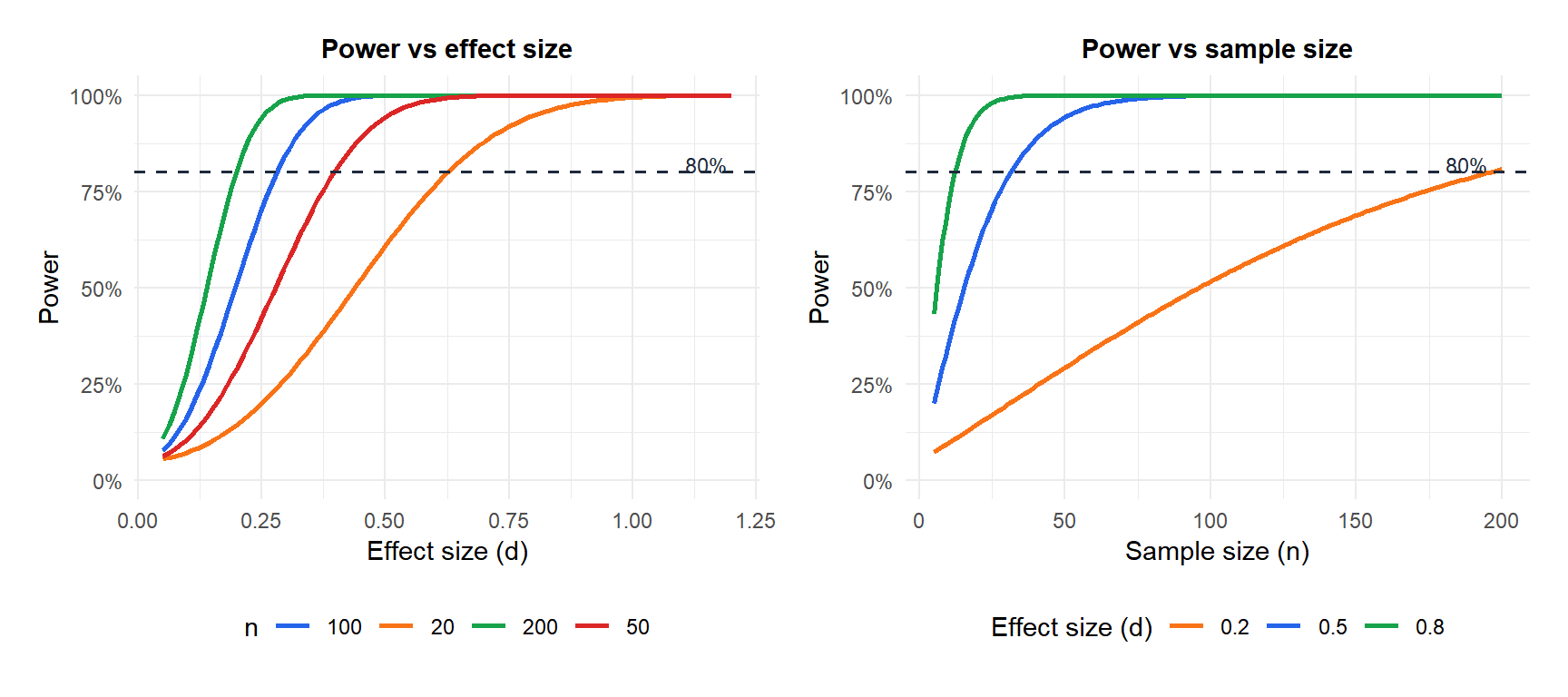
Visualizing power

Power is the area under the alternative distribution that falls in the rejection region. The following figure shows how it changes with effect size and sample size.

Calculating power for a one-sample z-test

For a two-sided one-sample z-test with known \(\sigma\), testing \(H_0: \mu = \mu_0\) vs \(H_1: \mu = \mu_1\):

\[\text{Power} = \Phi\!\left(\frac{|\mu_1 - \mu_0|}{\sigma/\sqrt{n}} - z_{\alpha/2}\right) + \Phi\!\left(-\frac{|\mu_1 - \mu_0|}{\sigma/\sqrt{n}} - z_{\alpha/2}\right)\]

where \(\Phi\) is the standard normal CDF. For practical purposes, the second term is negligible when the effect is not tiny, simplifying to:

\[\text{Power} \approx \Phi\!\left(\frac{|\mu_1 - \mu_0|}{\sigma/\sqrt{n}} - z_{\alpha/2}\right) = \Phi\!\left(d\sqrt{n} - z_{\alpha/2}\right)\]

where \(d = |\mu_1 - \mu_0|/\sigma\) is Cohen’s \(d\).

Calculating power: quality control

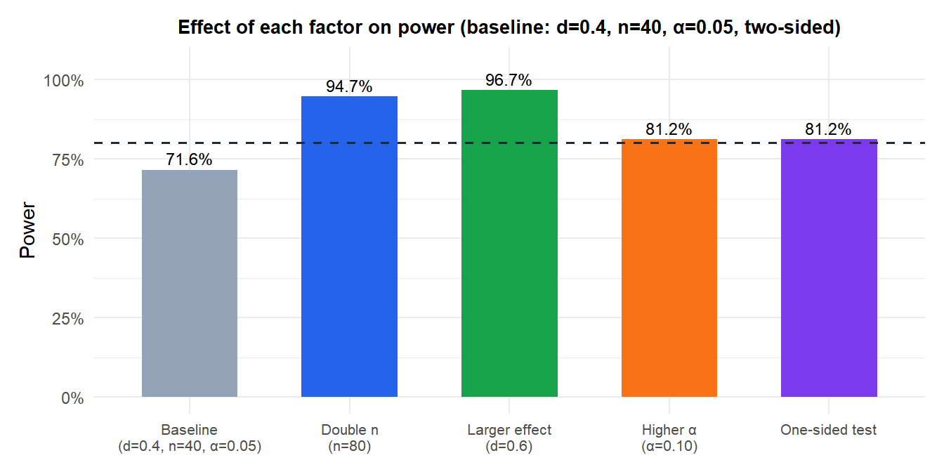
A factory monitors fill volume. \(H_0: \mu = 500\) ml. The process is considered problematic if \(\mu = 498\) ml (a 2 ml shift). Known \(\sigma = 5\) ml, \(n = 40\), \(\alpha = 0.05\).

\[d = \frac{|498 - 500|}{5} = 0.4, \qquad d\sqrt{n} = 0.4 \times \sqrt{40} \approx 2.530\]

\[\text{Power} \approx \Phi(2.530 - 1.960) = \Phi(0.570) \approx 0.716\]

The test has 71.6% power to detect a 2 ml shift with \(n = 40\). This is below the 80% target. To achieve 80% power:

\[n \geq \left(\frac{z_{0.025} + z_{0.20}}{d}\right)^2 = \left(\frac{1.960 + 0.842}{0.4}\right)^2 = \left(\frac{2.802}{0.4}\right)^2 \approx 49\]

With \(n = 49\) (round up to 50), the test achieves \(\geq 80\%\) power.

A priori vs post hoc power analysis

A priori power analysis

Conducted before data collection. You specify the desired power (e.g. 0.80), the significance level \(\alpha\), and the minimum effect size you want to detect, and solve for \(n\). This is the correct use of power analysis.

Post hoc (observed) power analysis

Conducted after the study, using the observed effect size and the actual \(n\) to compute power. This practice is almost always uninformative and often misleading.

Factors that increase power

Given a fixed effect size and \(\alpha\), power can be increased by:

• Increasing \(n\): the most direct lever.
• Reducing \(\sigma\): better measurement instruments, more homogeneous samples, controlling confounders.
• Using a one-sided test: if the direction is known in advance and justified, the critical value is smaller, increasing power. Use this only when appropriate.
• Increasing \(\alpha\): accepting a higher Type I error rate to reduce Type II errors. Justified when the cost of missing a real effect exceeds the cost of a false alarm (e.g. screening tests).
• Matched or paired designs: pairing removes between-subject variability, effectively reducing \(\sigma\).

Doubling \(n\) is the most reliable lever. Switching to a one-sided test gives a moderate boost but requires justification. Increasing \(\alpha\) trades Type I error for power.